This is “Elasticity: A Measure of Response”, chapter 5 from the book Microeconomics Principles (v. 2.0). For details on it (including licensing), click here.
For more information on the source of this book, or why it is available for free, please see the project's home page. You can browse or download additional books there. To download a .zip file containing this book to use offline, simply click here.


Chapter 5 Elasticity: A Measure of Response
Start Up: Raise Fares? Lower Fares? What’s a Public Transit Manager To Do?
Imagine that you are the manager of the public transportation system for a large metropolitan area. Operating costs for the system have soared in the last few years, and you are under pressure to boost revenues. What do you do?
An obvious choice would be to raise fares. That will make your customers angry, but at least it will generate the extra revenue you need—or will it? The law of demand says that raising fares will reduce the number of passengers riding on your system. If the number of passengers falls only a little, then the higher fares that your remaining passengers are paying might produce the higher revenues you need. But what if the number of passengers falls by so much that your higher fares actually reduce your revenues? If that happens, you will have made your customers mad and your financial problem worse!
Maybe you should recommend lower fares. After all, the law of demand also says that lower fares will increase the number of passengers. Having more people use the public transportation system could more than offset a lower fare you collect from each person. But it might not. What will you do?
Your job and the fiscal health of the public transit system are riding on your making the correct decision. To do so, you need to know just how responsive the quantity demanded is to a price change. You need a measure of responsiveness.
Economists use a measure of responsiveness called elasticity. ElasticityThe ratio of the percentage change in a dependent variable to a percentage change in an independent variable. is the ratio of the percentage change in a dependent variable to a percentage change in an independent variable. If the dependent variable is y, and the independent variable is x, then the elasticity of y with respect to a change in x is given by:
A variable such as y is said to be more elastic (responsive) if the percentage change in y is large relative to the percentage change in x. It is less elastic if the reverse is true.
As manager of the public transit system, for example, you will want to know how responsive the number of passengers on your system (the dependent variable) will be to a change in fares (the independent variable). The concept of elasticity will help you solve your public transit pricing problem and a great many other issues in economics. We will examine several elasticities in this chapter—all will tell us how responsive one variable is to a change in another.
5.1 The Price Elasticity of Demand
Learning Objectives
- Explain the concept of price elasticity of demand and its calculation.
- Explain what it means for demand to be price inelastic, unit price elastic, price elastic, perfectly price inelastic, and perfectly price elastic.
- Explain how and why the value of the price elasticity of demand changes along a linear demand curve.
- Understand the relationship between total revenue and price elasticity of demand.
- Discuss the determinants of price elasticity of demand.
We know from the law of demand how the quantity demanded will respond to a price change: it will change in the opposite direction. But how much will it change? It seems reasonable to expect, for example, that a 10% change in the price charged for a visit to the doctor would yield a different percentage change in quantity demanded than a 10% change in the price of a Ford Mustang. But how much is this difference?
To show how responsive quantity demanded is to a change in price, we apply the concept of elasticity. The price elasticity of demandThe percentage change in quantity demanded of a particular good or service divided by the percentage change in the price of that good or service, all other things unchanged. for a good or service, eD, is the percentage change in quantity demanded of a particular good or service divided by the percentage change in the price of that good or service, all other things unchanged. Thus we can write
Equation 5.1
Because the price elasticity of demand shows the responsiveness of quantity demanded to a price change, assuming that other factors that influence demand are unchanged, it reflects movements along a demand curve. With a downward-sloping demand curve, price and quantity demanded move in opposite directions, so the price elasticity of demand is always negative. A positive percentage change in price implies a negative percentage change in quantity demanded, and vice versa. Sometimes you will see the absolute value of the price elasticity measure reported. In essence, the minus sign is ignored because it is expected that there will be a negative (inverse) relationship between quantity demanded and price. In this text, however, we will retain the minus sign in reporting price elasticity of demand and will say “the absolute value of the price elasticity of demand” when that is what we are describing.
Heads Up!
Be careful not to confuse elasticity with slope. The slope of a line is the change in the value of the variable on the vertical axis divided by the change in the value of the variable on the horizontal axis between two points. Elasticity is the ratio of the percentage changes. The slope of a demand curve, for example, is the ratio of the change in price to the change in quantity between two points on the curve. The price elasticity of demand is the ratio of the percentage change in quantity to the percentage change in price. As we will see, when computing elasticity at different points on a linear demand curve, the slope is constant—that is, it does not change—but the value for elasticity will change.
Computing the Price Elasticity of Demand
Finding the price elasticity of demand requires that we first compute percentage changes in price and in quantity demanded. We calculate those changes between two points on a demand curve.
Figure 5.1 "Responsiveness and Demand" shows a particular demand curve, a linear demand curve for public transit rides. Suppose the initial price is $0.80, and the quantity demanded is 40,000 rides per day; we are at point A on the curve. Now suppose the price falls to $0.70, and we want to report the responsiveness of the quantity demanded. We see that at the new price, the quantity demanded rises to 60,000 rides per day (point B). To compute the elasticity, we need to compute the percentage changes in price and in quantity demanded between points A and B.
Figure 5.1 Responsiveness and Demand
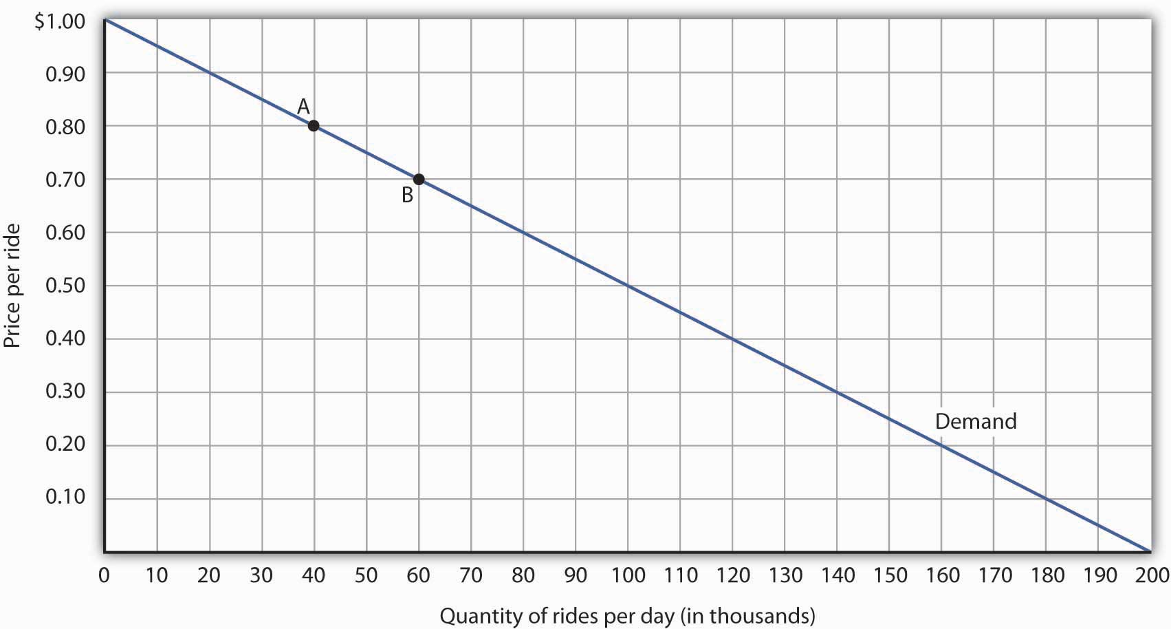
The demand curve shows how changes in price lead to changes in the quantity demanded. A movement from point A to point B shows that a $0.10 reduction in price increases the number of rides per day by 20,000. A movement from B to A is a $0.10 increase in price, which reduces quantity demanded by 20,000 rides per day.
We measure the percentage change between two points as the change in the variable divided by the average value of the variable between the two points. Thus, the percentage change in quantity between points A and B in Figure 5.1 "Responsiveness and Demand" is computed relative to the average of the quantity values at points A and B: (60,000 + 40,000)/2 = 50,000. The percentage change in quantity, then, is 20,000/50,000, or 40%. Likewise, the percentage change in price between points A and B is based on the average of the two prices: ($0.80 + $0.70)/2 = $0.75, and so we have a percentage change of −0.10/0.75, or −13.33%. The price elasticity of demand between points A and B is thus 40%/(−13.33%) = −3.00.
This measure of elasticity, which is based on percentage changes relative to the average value of each variable between two points, is called arc elasticityMeasure of elasticity based on percentage changes relative to the average value of each variable between two points.. The arc elasticity method has the advantage that it yields the same elasticity whether we go from point A to point B or from point B to point A. It is the method we shall use to compute elasticity.
For the arc elasticity method, we calculate the price elasticity of demand using the average value of price, , and the average value of quantity demanded, . We shall use the Greek letter Δ to mean “change in,” so the change in quantity between two points is ΔQ and the change in price is ΔP. Now we can write the formula for the price elasticity of demand as
Equation 5.2
The price elasticity of demand between points A and B is thus:
With the arc elasticity formula, the elasticity is the same whether we move from point A to point B or from point B to point A. If we start at point B and move to point A, we have:
The arc elasticity method gives us an estimate of elasticity. It gives the value of elasticity at the midpoint over a range of change, such as the movement between points A and B. For a precise computation of elasticity, we would need to consider the response of a dependent variable to an extremely small change in an independent variable. The fact that arc elasticities are approximate suggests an important practical rule in calculating arc elasticities: we should consider only small changes in independent variables. We cannot apply the concept of arc elasticity to large changes.
Another argument for considering only small changes in computing price elasticities of demand will become evident in the next section. We will investigate what happens to price elasticities as we move from one point to another along a linear demand curve.
Heads Up!
Notice that in the arc elasticity formula, the method for computing a percentage change differs from the standard method with which you may be familiar. That method measures the percentage change in a variable relative to its original value. For example, using the standard method, when we go from point A to point B, we would compute the percentage change in quantity as 20,000/40,000 = 50%. The percentage change in price would be −$0.10/$0.80 = −12.5%. The price elasticity of demand would then be 50%/(−12.5%) = −4.00. Going from point B to point A, however, would yield a different elasticity. The percentage change in quantity would be −20,000/60,000, or −33.33%. The percentage change in price would be $0.10/$0.70 = 14.29%. The price elasticity of demand would thus be −33.33%/14.29% = −2.33. By using the average quantity and average price to calculate percentage changes, the arc elasticity approach avoids the necessity to specify the direction of the change and, thereby, gives us the same answer whether we go from A to B or from B to A.
Price Elasticities Along a Linear Demand Curve
What happens to the price elasticity of demand when we travel along the demand curve? The answer depends on the nature of the demand curve itself. On a linear demand curve, such as the one in Figure 5.2 "Price Elasticities of Demand for a Linear Demand Curve", elasticity becomes smaller (in absolute value) as we travel downward and to the right.
Figure 5.2 Price Elasticities of Demand for a Linear Demand Curve
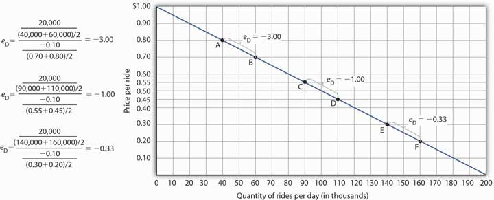
The price elasticity of demand varies between different pairs of points along a linear demand curve. The lower the price and the greater the quantity demanded, the lower the absolute value of the price elasticity of demand.
Figure 5.2 "Price Elasticities of Demand for a Linear Demand Curve" shows the same demand curve we saw in Figure 5.1 "Responsiveness and Demand". We have already calculated the price elasticity of demand between points A and B; it equals −3.00. Notice, however, that when we use the same method to compute the price elasticity of demand between other sets of points, our answer varies. For each of the pairs of points shown, the changes in price and quantity demanded are the same (a $0.10 decrease in price and 20,000 additional rides per day, respectively). But at the high prices and low quantities on the upper part of the demand curve, the percentage change in quantity is relatively large, whereas the percentage change in price is relatively small. The absolute value of the price elasticity of demand is thus relatively large. As we move down the demand curve, equal changes in quantity represent smaller and smaller percentage changes, whereas equal changes in price represent larger and larger percentage changes, and the absolute value of the elasticity measure declines. Between points C and D, for example, the price elasticity of demand is −1.00, and between points E and F the price elasticity of demand is −0.33.
On a linear demand curve, the price elasticity of demand varies depending on the interval over which we are measuring it. For any linear demand curve, the absolute value of the price elasticity of demand will fall as we move down and to the right along the curve.
The Price Elasticity of Demand and Changes in Total Revenue
Suppose the public transit authority is considering raising fares. Will its total revenues go up or down? Total revenueA firm’s output multiplied by the price at which it sells that output. is the price per unit times the number of units sold.Notice that since the number of units sold of a good is the same as the number of units bought, the definition for total revenue could also be used to define total spending. Which term we use depends on the question at hand. If we are trying to determine what happens to revenues of sellers, then we are asking about total revenue. If we are trying to determine how much consumers spend, then we are asking about total spending. In this case, it is the fare times the number of riders. The transit authority will certainly want to know whether a price increase will cause its total revenue to rise or fall. In fact, determining the impact of a price change on total revenue is crucial to the analysis of many problems in economics.
We will do two quick calculations before generalizing the principle involved. Given the demand curve shown in Figure 5.2 "Price Elasticities of Demand for a Linear Demand Curve", we see that at a price of $0.80, the transit authority will sell 40,000 rides per day. Total revenue would be $32,000 per day ($0.80 times 40,000). If the price were lowered by $0.10 to $0.70, quantity demanded would increase to 60,000 rides and total revenue would increase to $42,000 ($0.70 times 60,000). The reduction in fare increases total revenue. However, if the initial price had been $0.30 and the transit authority reduced it by $0.10 to $0.20, total revenue would decrease from $42,000 ($0.30 times 140,000) to $32,000 ($0.20 times 160,000). So it appears that the impact of a price change on total revenue depends on the initial price and, by implication, the original elasticity. We generalize this point in the remainder of this section.
The problem in assessing the impact of a price change on total revenue of a good or service is that a change in price always changes the quantity demanded in the opposite direction. An increase in price reduces the quantity demanded, and a reduction in price increases the quantity demanded. The question is how much. Because total revenue is found by multiplying the price per unit times the quantity demanded, it is not clear whether a change in price will cause total revenue to rise or fall.
We have already made this point in the context of the transit authority. Consider the following three examples of price increases for gasoline, pizza, and diet cola.
Suppose that 1,000 gallons of gasoline per day are demanded at a price of $4.00 per gallon. Total revenue for gasoline thus equals $4,000 per day (=1,000 gallons per day times $4.00 per gallon). If an increase in the price of gasoline to $4.25 reduces the quantity demanded to 950 gallons per day, total revenue rises to $4,037.50 per day (=950 gallons per day times $4.25 per gallon). Even though people consume less gasoline at $4.25 than at $4.00, total revenue rises because the higher price more than makes up for the drop in consumption.
Next consider pizza. Suppose 1,000 pizzas per week are demanded at a price of $9 per pizza. Total revenue for pizza equals $9,000 per week (=1,000 pizzas per week times $9 per pizza). If an increase in the price of pizza to $10 per pizza reduces quantity demanded to 900 pizzas per week, total revenue will still be $9,000 per week (=900 pizzas per week times $10 per pizza). Again, when price goes up, consumers buy less, but this time there is no change in total revenue.
Now consider diet cola. Suppose 1,000 cans of diet cola per day are demanded at a price of $0.50 per can. Total revenue for diet cola equals $500 per day (=1,000 cans per day times $0.50 per can). If an increase in the price of diet cola to $0.55 per can reduces quantity demanded to 880 cans per month, total revenue for diet cola falls to $484 per day (=880 cans per day times $0.55 per can). As in the case of gasoline, people will buy less diet cola when the price rises from $0.50 to $0.55, but in this example total revenue drops.
In our first example, an increase in price increased total revenue. In the second, a price increase left total revenue unchanged. In the third example, the price rise reduced total revenue. Is there a way to predict how a price change will affect total revenue? There is; the effect depends on the price elasticity of demand.
Elastic, Unit Elastic, and Inelastic Demand
To determine how a price change will affect total revenue, economists place price elasticities of demand in three categories, based on their absolute value. If the absolute value of the price elasticity of demand is greater than 1, demand is termed price elasticSituation in which the absolute value of the price elasticity of demand is greater than 1.. If it is equal to 1, demand is unit price elasticSituation in which the absolute value of the price elasticity of demand is equal to 1.. And if it is less than 1, demand is price inelasticSituation in which the absolute value of the price of elasticity of demand is less than 1..
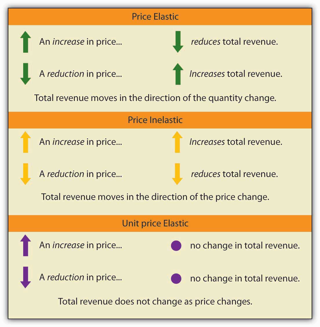
Relating Elasticity to Changes in Total Revenue
When the price of a good or service changes, the quantity demanded changes in the opposite direction. Total revenue will move in the direction of the variable that changes by the larger percentage. If the variables move by the same percentage, total revenue stays the same. If quantity demanded changes by a larger percentage than price (i.e., if demand is price elastic), total revenue will change in the direction of the quantity change. If price changes by a larger percentage than quantity demanded (i.e., if demand is price inelastic), total revenue will move in the direction of the price change. If price and quantity demanded change by the same percentage (i.e., if demand is unit price elastic), then total revenue does not change.
When demand is price inelastic, a given percentage change in price results in a smaller percentage change in quantity demanded. That implies that total revenue will move in the direction of the price change: a reduction in price will reduce total revenue, and an increase in price will increase it.
Consider the price elasticity of demand for gasoline. In the example above, 1,000 gallons of gasoline were purchased each day at a price of $4.00 per gallon; an increase in price to $4.25 per gallon reduced the quantity demanded to 950 gallons per day. We thus had an average quantity of 975 gallons per day and an average price of $4.125. We can thus calculate the arc price elasticity of demand for gasoline:
The demand for gasoline is price inelastic, and total revenue moves in the direction of the price change. When price rises, total revenue rises. Recall that in our example above, total spending on gasoline (which equals total revenues to sellers) rose from $4,000 per day (=1,000 gallons per day times $4.00) to $4037.50 per day (=950 gallons per day times $4.25 per gallon).
When demand is price inelastic, a given percentage change in price results in a smaller percentage change in quantity demanded. That implies that total revenue will move in the direction of the price change: an increase in price will increase total revenue, and a reduction in price will reduce it.
Consider again the example of pizza that we examined above. At a price of $9 per pizza, 1,000 pizzas per week were demanded. Total revenue was $9,000 per week (=1,000 pizzas per week times $9 per pizza). When the price rose to $10, the quantity demanded fell to 900 pizzas per week. Total revenue remained $9,000 per week (=900 pizzas per week times $10 per pizza). Again, we have an average quantity of 950 pizzas per week and an average price of $9.50. Using the arc elasticity method, we can compute:
Demand is unit price elastic, and total revenue remains unchanged. Quantity demanded falls by the same percentage by which price increases.
Consider next the example of diet cola demand. At a price of $0.50 per can, 1,000 cans of diet cola were purchased each day. Total revenue was thus $500 per day (=$0.50 per can times 1,000 cans per day). An increase in price to $0.55 reduced the quantity demanded to 880 cans per day. We thus have an average quantity of 940 cans per day and an average price of $0.525 per can. Computing the price elasticity of demand for diet cola in this example, we have:
The demand for diet cola is price elastic, so total revenue moves in the direction of the quantity change. It falls from $500 per day before the price increase to $484 per day after the price increase.
A demand curve can also be used to show changes in total revenue. Figure 5.3 "Changes in Total Revenue and a Linear Demand Curve" shows the demand curve from Figure 5.1 "Responsiveness and Demand" and Figure 5.2 "Price Elasticities of Demand for a Linear Demand Curve". At point A, total revenue from public transit rides is given by the area of a rectangle drawn with point A in the upper right-hand corner and the origin in the lower left-hand corner. The height of the rectangle is price; its width is quantity. We have already seen that total revenue at point A is $32,000 ($0.80 × 40,000). When we reduce the price and move to point B, the rectangle showing total revenue becomes shorter and wider. Notice that the area gained in moving to the rectangle at B is greater than the area lost; total revenue rises to $42,000 ($0.70 × 60,000). Recall from Figure 5.2 "Price Elasticities of Demand for a Linear Demand Curve" that demand is elastic between points A and B. In general, demand is elastic in the upper half of any linear demand curve, so total revenue moves in the direction of the quantity change.
Figure 5.3 Changes in Total Revenue and a Linear Demand Curve

Moving from point A to point B implies a reduction in price and an increase in the quantity demanded. Demand is elastic between these two points. Total revenue, shown by the areas of the rectangles drawn from points A and B to the origin, rises. When we move from point E to point F, which is in the inelastic region of the demand curve, total revenue falls.
A movement from point E to point F also shows a reduction in price and an increase in quantity demanded. This time, however, we are in an inelastic region of the demand curve. Total revenue now moves in the direction of the price change—it falls. Notice that the rectangle drawn from point F is smaller in area than the rectangle drawn from point E, once again confirming our earlier calculation.
We have noted that a linear demand curve is more elastic where prices are relatively high and quantities relatively low and less elastic where prices are relatively low and quantities relatively high. We can be even more specific. For any linear demand curve, demand will be price elastic in the upper half of the curve and price inelastic in its lower half. At the midpoint of a linear demand curve, demand is unit price elastic.
Constant Price Elasticity of Demand Curves
Figure 5.4 "Demand Curves with Constant Price Elasticities" shows four demand curves over which price elasticity of demand is the same at all points. The demand curve in Panel (a) is vertical. This means that price changes have no effect on quantity demanded. The numerator of the formula given in Equation 5.1 for the price elasticity of demand (percentage change in quantity demanded) is zero. The price elasticity of demand in this case is therefore zero, and the demand curve is said to be perfectly inelasticSituation in which the price elasticity of demand is zero.. This is a theoretically extreme case, and no good that has been studied empirically exactly fits it. A good that comes close, at least over a specific price range, is insulin. A diabetic will not consume more insulin as its price falls but, over some price range, will consume the amount needed to control the disease.
Figure 5.4 Demand Curves with Constant Price Elasticities
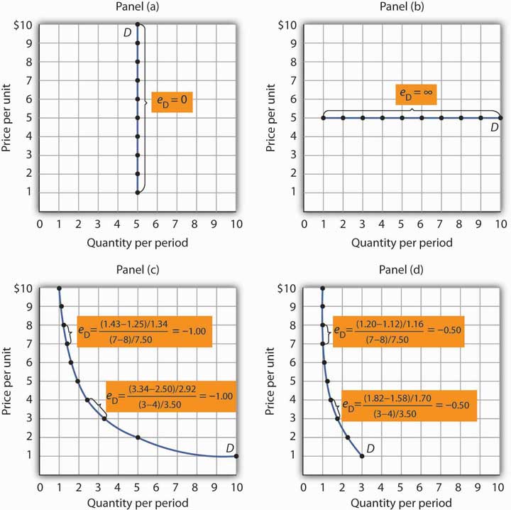
The demand curve in Panel (a) is perfectly inelastic. The demand curve in Panel (b) is perfectly elastic. Price elasticity of demand is −1.00 all along the demand curve in Panel (c), whereas it is −0.50 all along the demand curve in Panel (d).
As illustrated in Figure 5.4 "Demand Curves with Constant Price Elasticities", several other types of demand curves have the same elasticity at every point on them. The demand curve in Panel (b) is horizontal. This means that even the smallest price changes have enormous effects on quantity demanded. The denominator of the formula given in Equation 5.1 for the price elasticity of demand (percentage change in price) approaches zero. The price elasticity of demand in this case is therefore infinite, and the demand curve is said to be perfectly elasticSituation in which the price elasticity of demand is infinite..Division by zero results in an undefined solution. Saying that the price elasticity of demand is infinite requires that we say the denominator “approaches” zero. This is the type of demand curve faced by producers of standardized products such as wheat. If the wheat of other farms is selling at $4 per bushel, a typical farm can sell as much wheat as it wants to at $4 but nothing at a higher price and would have no reason to offer its wheat at a lower price.
The nonlinear demand curves in Panels (c) and (d) have price elasticities of demand that are negative; but, unlike the linear demand curve discussed above, the value of the price elasticity is constant all along each demand curve. The demand curve in Panel (c) has price elasticity of demand equal to −1.00 throughout its range; in Panel (d) the price elasticity of demand is equal to −0.50 throughout its range. Empirical estimates of demand often show curves like those in Panels (c) and (d) that have the same elasticity at every point on the curve.
Heads Up!
Do not confuse price inelastic demand and perfectly inelastic demand. Perfectly inelastic demand means that the change in quantity is zero for any percentage change in price; the demand curve in this case is vertical. Price inelastic demand means only that the percentage change in quantity is less than the percentage change in price, not that the change in quantity is zero. With price inelastic (as opposed to perfectly inelastic) demand, the demand curve itself is still downward sloping.
Determinants of the Price Elasticity of Demand
The greater the absolute value of the price elasticity of demand, the greater the responsiveness of quantity demanded to a price change. What determines whether demand is more or less price elastic? The most important determinants of the price elasticity of demand for a good or service are the availability of substitutes, the importance of the item in household budgets, and time.
Availability of Substitutes
The price elasticity of demand for a good or service will be greater in absolute value if many close substitutes are available for it. If there are lots of substitutes for a particular good or service, then it is easy for consumers to switch to those substitutes when there is a price increase for that good or service. Suppose, for example, that the price of Ford automobiles goes up. There are many close substitutes for Fords—Chevrolets, Chryslers, Toyotas, and so on. The availability of close substitutes tends to make the demand for Fords more price elastic.
If a good has no close substitutes, its demand is likely to be somewhat less price elastic. There are no close substitutes for gasoline, for example. The price elasticity of demand for gasoline in the intermediate term of, say, three–nine months is generally estimated to be about −0.5. Since the absolute value of price elasticity is less than 1, it is price inelastic. We would expect, though, that the demand for a particular brand of gasoline will be much more price elastic than the demand for gasoline in general.
Importance in Household Budgets
One reason price changes affect quantity demanded is that they change how much a consumer can buy; a change in the price of a good or service affects the purchasing power of a consumer’s income and thus affects the amount of a good the consumer will buy. This effect is stronger when a good or service is important in a typical household’s budget.
A change in the price of jeans, for example, is probably more important in your budget than a change in the price of pencils. Suppose the prices of both were to double. You had planned to buy four pairs of jeans this year, but now you might decide to make do with two new pairs. A change in pencil prices, in contrast, might lead to very little reduction in quantity demanded simply because pencils are not likely to loom large in household budgets. The greater the importance of an item in household budgets, the greater the absolute value of the price elasticity of demand is likely to be.
Time
Suppose the price of electricity rises tomorrow morning. What will happen to the quantity demanded?
The answer depends in large part on how much time we allow for a response. If we are interested in the reduction in quantity demanded by tomorrow afternoon, we can expect that the response will be very small. But if we give consumers a year to respond to the price change, we can expect the response to be much greater. We expect that the absolute value of the price elasticity of demand will be greater when more time is allowed for consumer responses.
Consider the price elasticity of crude oil demand. Economist John C. B. Cooper estimated short- and long-run price elasticities of demand for crude oil for 23 industrialized nations for the period 1971–2000. Professor Cooper found that for virtually every country, the price elasticities were negative, and the long-run price elasticities were generally much greater (in absolute value) than were the short-run price elasticities. His results are reported in Table 5.1 "Short- and Long-Run Price Elasticities of the Demand for Crude Oil in 23 Countries". As you can see, the research was reported in a journal published by OPEC (Organization of Petroleum Exporting Countries), an organization whose members have profited greatly from the inelasticity of demand for their product. By restricting supply, OPEC, which produces about 45% of the world’s crude oil, is able to put upward pressure on the price of crude. That increases OPEC’s (and all other oil producers’) total revenues and reduces total costs.
Table 5.1 Short- and Long-Run Price Elasticities of the Demand for Crude Oil in 23 Countries
| Country | Short-Run Price Elasticity of Demand | Long-Run Price Elasticity of Demand |
|---|---|---|
| Australia | −0.034 | −0.068 |
| Austria | −0.059 | −0.092 |
| Canada | −0.041 | −0.352 |
| China | 0.001 | 0.005 |
| Denmark | −0.026 | −0.191 |
| Finland | −0.016 | −0.033 |
| France | −0.069 | −0.568 |
| Germany | −0.024 | −0.279 |
| Greece | −0.055 | −0.126 |
| Iceland | −0.109 | −0.452 |
| Ireland | −0.082 | −0.196 |
| Italy | −0.035 | −0.208 |
| Japan | −0.071 | −0.357 |
| Korea | −0.094 | −0.178 |
| Netherlands | −0.057 | −0.244 |
| New Zealand | −0.054 | −0.326 |
| Norway | −0.026 | −0.036 |
| Portugal | 0.023 | 0.038 |
| Spain | −0.087 | −0.146 |
| Sweden | −0.043 | −0.289 |
| Switzerland | −0.030 | −0.056 |
| United Kingdom | −0.068 | −0.182 |
| United States | −0.061 | −0.453 |
For most countries, price elasticity of demand for crude oil tends to be greater (in absolute value) in the long run than in the short run.
Source: John C. B. Cooper, “Price Elasticity of Demand for Crude Oil: Estimates from 23 Countries,” OPEC Review: Energy Economics & Related Issues 27:1 (March 2003): 4. The estimates are based on data for the period 1971–2000, except for China and South Korea, where the period is 1979–2000. While the price elasticities for China and Portugal were positive, they were not statistically significant.
Key Takeaways
- The price elasticity of demand measures the responsiveness of quantity demanded to changes in price; it is calculated by dividing the percentage change in quantity demanded by the percentage change in price.
- Demand is price inelastic if the absolute value of the price elasticity of demand is less than 1; it is unit price elastic if the absolute value is equal to 1; and it is price elastic if the absolute value is greater than 1.
- Demand is price elastic in the upper half of any linear demand curve and price inelastic in the lower half. It is unit price elastic at the midpoint.
- When demand is price inelastic, total revenue moves in the direction of a price change. When demand is unit price elastic, total revenue does not change in response to a price change. When demand is price elastic, total revenue moves in the direction of a quantity change.
- The absolute value of the price elasticity of demand is greater when substitutes are available, when the good is important in household budgets, and when buyers have more time to adjust to changes in the price of the good.
Try It!
You are now ready to play the part of the manager of the public transit system. Your finance officer has just advised you that the system faces a deficit. Your board does not want you to cut service, which means that you cannot cut costs. Your only hope is to increase revenue. Would a fare increase boost revenue?
You consult the economist on your staff who has researched studies on public transportation elasticities. She reports that the estimated price elasticity of demand for the first few months after a price change is about −0.3, but that after several years, it will be about −1.5.
- Explain why the estimated values for price elasticity of demand differ.
- Compute what will happen to ridership and revenue over the next few months if you decide to raise fares by 5%.
- Compute what will happen to ridership and revenue over the next few years if you decide to raise fares by 5%.
- What happens to total revenue now and after several years if you choose to raise fares?
Case in Point: Elasticity and Stop Lights

© 2010 Jupiterimages Corporation
We all face the situation every day. You are approaching an intersection. The yellow light comes on. You know that you are supposed to slow down, but you are in a bit of a hurry. So, you speed up a little to try to make the light. But the red light flashes on just before you get to the intersection. Should you risk it and go through?
Many people faced with that situation take the risky choice. In 1998, 2,000 people in the United States died as a result of drivers running red lights at intersections. In an effort to reduce the number of drivers who make such choices, many areas have installed cameras at intersections. Drivers who run red lights have their pictures taken and receive citations in the mail. This enforcement method, together with recent increases in the fines for driving through red lights at intersections, has led to an intriguing application of the concept of elasticity. Economists Avner Bar-Ilan of the University of Haifa in Israel and Bruce Sacerdote of Dartmouth University have estimated what is, in effect, the price elasticity for driving through stoplights with respect to traffic fines at intersections in Israel and in San Francisco.
In December 1996, Israel sharply increased the fine for driving through a red light. The old fine of 400 shekels (this was equal at that time to $122 in the United States) was increased to 1,000 shekels ($305). In January 1998, California raised its fine for the offense from $104 to $271. The country of Israel and the city of San Francisco installed cameras at several intersections. Drivers who ignored stoplights got their pictures taken and automatically received citations imposing the new higher fines.
We can think of driving through red lights as an activity for which there is a demand—after all, ignoring a red light speeds up one’s trip. It may also generate satisfaction to people who enjoy disobeying traffic laws. The concept of elasticity gives us a way to show just how responsive drivers were to the increase in fines.
Professors Bar-Ilan and Sacerdote obtained information on all the drivers cited at 73 intersections in Israel and eight intersections in San Francisco. For Israel, for example, they defined the period January 1992 to June 1996 as the “before” period. They compared the number of violations during the before period to the number of violations from July 1996 to December 1999—the “after” period—and found there was a reduction in tickets per driver of 31.5 per cent. Specifically, the average number of tickets per driver was 0.073 during the period before the increase; it fell to 0.050 after the increase. The increase in the fine was 150 per cent. (Note that, because they were making a “before” and “after” calculation, the authors used the standard method described in the Heads Up! on computing a percentage change—i.e., they computed the percentage changes in comparison to the original values instead of the average value of the variables.) The elasticity of citations with respect to the fine was thus −0.21 (= −31.5%/150%).
The economists estimated elasticities for particular groups of people. For example, young people (age 17–30) had an elasticity of −0.36; people over the age of 30 had an elasticity of −0.16. In general, elasticities fell in absolute value as income rose. For San Francisco and Israel combined, the elasticity was between −0.26 and −0.33.
In general, the results showed that people responded rationally to the increases in fines. Increasing the price of a particular behavior reduced the frequency of that behavior. The study also points out the effectiveness of cameras as an enforcement technique. With cameras, violators can be certain they will be cited if they ignore a red light. And reducing the number of people running red lights clearly saves lives.
Source: Avner Bar-Ilan and Bruce Sacerdote. “The Response of Criminals and Non-Criminals to Fines.” Journal of Law and Economics, 47:1 (April 2004): 1–17.
Answers to Try It! Problems
- The absolute value of price elasticity of demand tends to be greater when more time is allowed for consumers to respond. Over time, riders of the commuter rail system can organize car pools, move, or otherwise adjust to the fare increase.
- Using the formula for price elasticity of demand and plugging in values for the estimate of price elasticity (−0.5) and the percentage change in price (5%) and then rearranging terms, we can solve for the percentage change in quantity demanded as: eD = %Δ in Q/%Δ in P; −0.5 = %Δ in Q/5%; (−0.5)(5%) = %Δ in Q = −2.5%. Ridership falls by 2.5% in the first few months.
- Using the formula for price elasticity of demand and plugging in values for the estimate of price elasticity over a few years (−1.5) and the percentage change in price (5%), we can solve for the percentage change in quantity demanded as eD = %Δ in Q/%Δ in P ; −1.5 = %Δ in Q/5%; (−1.5)(5%) = %Δ in Q = −7.5%. Ridership falls by 7.5% over a few years.
- Total revenue rises immediately after the fare increase, since demand over the immediate period is price inelastic. Total revenue falls after a few years, since demand changes and becomes price elastic.
5.2 Responsiveness of Demand to Other Factors
Learning Objectives
- Explain the concept of income elasticity of demand and its calculation.
- Classify goods as normal or inferior depending on their income elasticity of demand.
- Explain the concept of cross price elasticity of demand and its calculation.
- Classify goods as substitutes or complements depending on their cross price elasticity of demand.
Although the response of quantity demanded to changes in price is the most widely used measure of elasticity, economists are interested in the response to changes in the demand shifters as well. Two of the most important measures show how demand responds to changes in income and to changes in the prices of related goods and services.
Income Elasticity of Demand
We saw in the chapter that introduced the model of demand and supply that the demand for a good or service is affected by income. We measure the income elasticity of demandThe percentage change in quantity demanded at a specific price divided by the percentage change in income that produced the demand change, all other things unchanged., eY, as the percentage change in quantity demanded at a specific price divided by the percentage change in income that produced the demand change, all other things unchanged:
Equation 5.3
The symbol Y is often used in economics to represent income. Because income elasticity of demand reports the responsiveness of quantity demanded to a change in income, all other things unchanged (including the price of the good), it reflects a shift in the demand curve at a given price. Remember that price elasticity of demand reflects movements along a demand curve in response to a change in price.
A positive income elasticity of demand means that income and demand move in the same direction—an increase in income increases demand, and a reduction in income reduces demand. As we learned, a good whose demand rises as income rises is called a normal good.
Studies show that most goods and services are normal, and thus their income elasticities are positive. Goods and services for which demand is likely to move in the same direction as income include housing, seafood, rock concerts, and medical services.
If a good or service is inferior, then an increase in income reduces demand for the good. That implies a negative income elasticity of demand. Goods and services for which the income elasticity of demand is likely to be negative include used clothing, beans, and urban public transit. For example, the studies we have already cited concerning the demands for urban public transit in France and in Madrid found the long-run income elasticities of demand to be negative (−0.23 in France and −0.25 in Madrid).See Georges Bresson, Joyce Dargay, Jean-Loup Madre, and Alain Pirotte, “Economic and Structural Determinants of the Demand for French Transport: An Analysis on a Panel of French Urban Areas Using Shrinkage Estimators.” Transportation Research: Part A 38: 4 (May 2004): 269–285. See also Anna Matas. “Demand and Revenue Implications of an Integrated Transport Policy: The Case of Madrid.” Transport Reviews 24:2 (March 2004): 195–217.
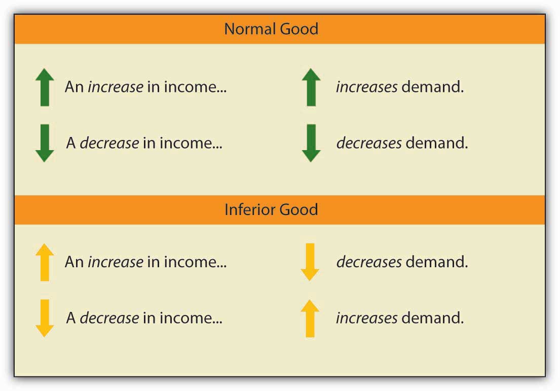
When we compute the income elasticity of demand, we are looking at the change in the quantity demanded at a specific price. We are thus dealing with a change that shifts the demand curve. An increase in income shifts the demand for a normal good to the right; it shifts the demand for an inferior good to the left.
Cross Price Elasticity of Demand
The demand for a good or service is affected by the prices of related goods or services. A reduction in the price of salsa, for example, would increase the demand for chips, suggesting that salsa is a complement of chips. A reduction in the price of chips, however, would reduce the demand for peanuts, suggesting that chips are a substitute for peanuts.
The measure economists use to describe the responsiveness of demand for a good or service to a change in the price of another good or service is called the cross price elasticity of demandIt equals the percentage change in the quantity demanded of one good or service at a specific price divided by the percentage change in the price of a related good or service., eA, B. It equals the percentage change in the quantity demanded of one good or service at a specific price divided by the percentage change in the price of a related good or service. We are varying the price of a related good when we consider the cross price elasticity of demand, so the response of quantity demanded is shown as a shift in the demand curve.
The cross price elasticity of the demand for good A with respect to the price of good B is given by:
Equation 5.4
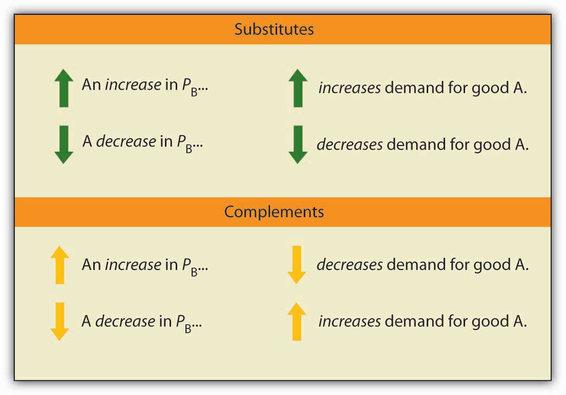
Cross price elasticities of demand define whether two goods are substitutes, complements, or unrelated. If two goods are substitutes, an increase in the price of one will lead to an increase in the demand for the other—the cross price elasticity of demand is positive. If two goods are complements, an increase in the price of one will lead to a reduction in the demand for the other—the cross price elasticity of demand is negative. If two goods are unrelated, a change in the price of one will not affect the demand for the other—the cross price elasticity of demand is zero.
An examination of the demand for local television advertising with respect to the price of local radio advertising revealed that the two goods are clearly substitutes. A 10 per cent increase in the price of local radio advertising led to a 10 per cent increase in demand for local television advertising, so that the cross price elasticity of demand for local television advertising with respect to changes in the price of radio advertising was 1.0.Robert B. Ekelund, S. Ford, and John D. Jackson. “Are Local TV Markets Separate Markets?” International Journal of the Economics of Business 7:1 (2000): 79–97.
Heads Up!
Notice that with income elasticity of demand and cross price elasticity of demand we are primarily concerned with whether the measured value of these elasticities is positive or negative. In the case of income elasticity of demand this tells us whether the good or service is normal or inferior. In the case of cross price elasticity of demand it tells us whether two goods are substitutes or complements. With price elasticity of demand we were concerned with whether the measured absolute value of this elasticity was greater than, less than, or equal to 1, because this gave us information about what happens to total revenue as price changes. The terms elastic and inelastic apply to price elasticity of demand. They are not used to describe income elasticity of demand or cross price elasticity of demand.
Key Takeaways
- The income elasticity of demand reflects the responsiveness of demand to changes in income. It is the percentage change in quantity demanded at a specific price divided by the percentage change in income, ceteris paribus.
- Income elasticity is positive for normal goods and negative for inferior goods.
- The cross price elasticity of demand measures the way demand for one good or service responds to changes in the price of another. It is the percentage change in the quantity demanded of one good or service at a specific price divided by the percentage change in the price of another good or service, all other things unchanged.
- Cross price elasticity is positive for substitutes, negative for complements, and zero for goods or services whose demands are unrelated.
Try It!
Suppose that when the price of bagels rises by 10%, the demand for cream cheese falls by 3% at the current price, and that when income rises by 10%, the demand for bagels increases by 1% at the current price. Calculate the cross price elasticity of demand for cream cheese with respect to the price of bagels and tell whether bagels and cream cheese are substitutes or complements. Calculate the income elasticity of demand and tell whether bagels are normal or inferior.
Case in Point: Various Demand Elasticities for Conventional and Organic Milk

© Thinkstock
Peruse the milk display at any supermarket and you will see a number of items that you would not have seen a decade ago. Choices include fat content; with or without lactose; animal milks or milk substitutes, such as soy or almond milk; flavors; and organic or conventional milk. Whereas in the 1990s only specialty stores stocked organic milk, today it is readily available in most supermarkets. In fact, the market share for organic milk has grown, as sales of conventional milk have been fairly constant while sales of organic milk have increased.
Professors Pedro Alviola and Oral Capps have estimated various demand elasticities associated with conventional and organic milk, based on a study of 38,000 households. Their results are summarized in the following table.
| Elasticity Measure | Organic Milk | Conventional Milk |
|---|---|---|
| Own-price elasticity | −2.00 | −0.87 |
| Cross-price elasticity | 0.70 | 0.18 |
| Income elasticity | 0.27 | −0.01 |
Organic milk is price elastic, while conventional milk is price inelastic. Both cross-price elasticities are positive, indicating that these two kinds of milk are substitutes but their estimated values differ. In particular, a 1% increase in the price of conventional milk leads to a 0.70% increase in the quantity demanded of organic milk, while a 1% increase in the price of organic milk leads to an increase in the quantity demanded of conventional milk of only 0.18%. This asymmetry suggests that organic milk consumers have considerable reluctance in switching back to what they may perceive as a lower-quality product. Finally, the income elasticity estimates suggest that organic milk is a normal good, while conventional milk is an inferior good. As might be expected, in the sample used in the study, purchasers of organic milk are more affluent as a group than are purchasers of conventional milk.
Being a fairly new product, organic milk studies are just becoming available and the authors point out that other researchers using different data sets have calculated different values for these elasticities. Over time, as more data become available and various studies are compared, this type of work is likely to influence milk marketing and pricing.
Source: Pedro A. Alviola IV and Oral Capps Jr., “Household Demand Analysis of Organic and Conventional Fluid Milk in the United States Based on the 2004 Nielsen Homescan Panel,” Agribusiness 26:3 (2010): 369–388.
Answer to Try It! Problem
Using the formula for cross price elasticity of demand, we find that eAB = (−3%)/(10%) = −0.3. Since the eAB is negative, bagels and cream cheese are complements. Using the formula for income elasticity of demand, we find that eY = (+1%)/(10%) = +0.1. Since eY is positive, bagels are a normal good.
5.3 Price Elasticity of Supply
Learning Objectives
- Explain the concept of elasticity of supply and its calculation.
- Explain what it means for supply to be price inelastic, unit price elastic, price elastic, perfectly price inelastic, and perfectly price elastic.
- Explain why time is an important determinant of price elasticity of supply.
- Apply the concept of price elasticity of supply to the labor supply curve.
The elasticity measures encountered so far in this chapter all relate to the demand side of the market. It is also useful to know how responsive quantity supplied is to a change in price.
Suppose the demand for apartments rises. There will be a shortage of apartments at the old level of apartment rents and pressure on rents to rise. All other things unchanged, the more responsive the quantity of apartments supplied is to changes in monthly rents, the lower the increase in rent required to eliminate the shortage and to bring the market back to equilibrium. Conversely, if quantity supplied is less responsive to price changes, price will have to rise more to eliminate a shortage caused by an increase in demand.
This is illustrated in Figure 5.5 "Increase in Apartment Rents Depends on How Responsive Supply Is". Suppose the rent for a typical apartment had been R0 and the quantity Q0 when the demand curve was D1 and the supply curve was either S1 (a supply curve in which quantity supplied is less responsive to price changes) or S2 (a supply curve in which quantity supplied is more responsive to price changes). Note that with either supply curve, equilibrium price and quantity are initially the same. Now suppose that demand increases to D2, perhaps due to population growth. With supply curve S1, the price (rent in this case) will rise to R1 and the quantity of apartments will rise to Q1. If, however, the supply curve had been S2, the rent would only have to rise to R2 to bring the market back to equilibrium. In addition, the new equilibrium number of apartments would be higher at Q2. Supply curve S2 shows greater responsiveness of quantity supplied to price change than does supply curve S1.
Figure 5.5 Increase in Apartment Rents Depends on How Responsive Supply Is
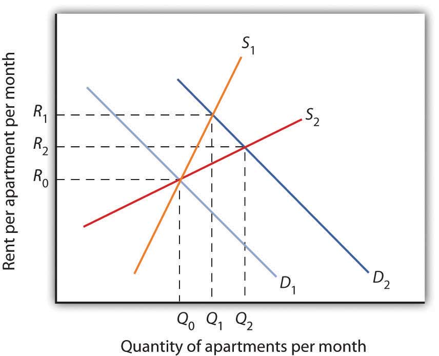
The more responsive the supply of apartments is to changes in price (rent in this case), the less rents rise when the demand for apartments increases.
We measure the price elasticity of supplyThe ratio of the percentage change in quantity supplied of a good or service to the percentage change in its price, all other things unchanged. (eS) as the ratio of the percentage change in quantity supplied of a good or service to the percentage change in its price, all other things unchanged:
Equation 5.5
Because price and quantity supplied usually move in the same direction, the price elasticity of supply is usually positive. The larger the price elasticity of supply, the more responsive the firms that supply the good or service are to a price change.
Supply is price elastic if the price elasticity of supply is greater than 1, unit price elastic if it is equal to 1, and price inelastic if it is less than 1. A vertical supply curve, as shown in Panel (a) of Figure 5.6 "Supply Curves and Their Price Elasticities", is perfectly inelastic; its price elasticity of supply is zero. The supply of Beatles’ songs is perfectly inelastic because the band no longer exists. A horizontal supply curve, as shown in Panel (b) of Figure 5.6 "Supply Curves and Their Price Elasticities", is perfectly elastic; its price elasticity of supply is infinite. It means that suppliers are willing to supply any amount at a certain price.
Figure 5.6 Supply Curves and Their Price Elasticities
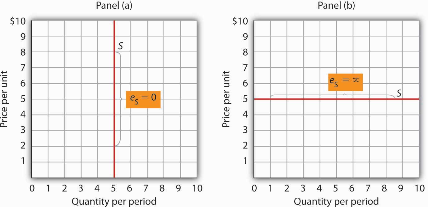
The supply curve in Panel (a) is perfectly inelastic. In Panel (b), the supply curve is perfectly elastic.
Time: An Important Determinant of the Elasticity of Supply
Time plays a very important role in the determination of the price elasticity of supply. Look again at the effect of rent increases on the supply of apartments. Suppose apartment rents in a city rise. If we are looking at a supply curve of apartments over a period of a few months, the rent increase is likely to induce apartment owners to rent out a relatively small number of additional apartments. With the higher rents, apartment owners may be more vigorous in reducing their vacancy rates, and, indeed, with more people looking for apartments to rent, this should be fairly easy to accomplish. Attics and basements are easy to renovate and rent out as additional units. In a short period of time, however, the supply response is likely to be fairly modest, implying that the price elasticity of supply is fairly low. A supply curve corresponding to a short period of time would look like S1 in Figure 5.5 "Increase in Apartment Rents Depends on How Responsive Supply Is". It is during such periods that there may be calls for rent controls.
If the period of time under consideration is a few years rather than a few months, the supply curve is likely to be much more price elastic. Over time, buildings can be converted from other uses and new apartment complexes can be built. A supply curve corresponding to a longer period of time would look like S2 in Figure 5.5 "Increase in Apartment Rents Depends on How Responsive Supply Is".
Elasticity of Labor Supply: A Special Application
The concept of price elasticity of supply can be applied to labor to show how the quantity of labor supplied responds to changes in wages or salaries. What makes this case interesting is that it has sometimes been found that the measured elasticity is negative, that is, that an increase in the wage rate is associated with a reduction in the quantity of labor supplied.
In most cases, labor supply curves have their normal upward slope: higher wages induce people to work more. For them, having the additional income from working more is preferable to having more leisure time. However, wage increases may lead some people in very highly paid jobs to cut back on the number of hours they work because their incomes are already high and they would rather have more time for leisure activities. In this case, the labor supply curve would have a negative slope. The reasons for this phenomenon are explained more fully in a later chapter. The Case in Point in this section gives another example where an increase in the wage may reduce the number of hours of work.
Key Takeaways
- The price elasticity of supply measures the responsiveness of quantity supplied to changes in price. It is the percentage change in quantity supplied divided by the percentage change in price. It is usually positive.
- Supply is price inelastic if the price elasticity of supply is less than 1; it is unit price elastic if the price elasticity of supply is equal to 1; and it is price elastic if the price elasticity of supply is greater than 1. A vertical supply curve is said to be perfectly inelastic. A horizontal supply curve is said to be perfectly elastic.
- The price elasticity of supply is greater when the length of time under consideration is longer because over time producers have more options for adjusting to the change in price.
- When applied to labor supply, the price elasticity of supply is usually positive but can be negative. If higher wages induce people to work more, the labor supply curve is upward sloping and the price elasticity of supply is positive. In some very high-paying professions or other unusual circumstances, the labor supply curve may have a negative slope, which leads to a negative price elasticity of supply.
Try It!
In the late 1990s, it was reported on the news that the high-tech industry was worried about being able to find enough workers with computer-related expertise. Job offers for recent college graduates with degrees in computer science went with high salaries. It was also reported that more undergraduates than ever were majoring in computer science. Compare the price elasticity of supply of computer scientists at that point in time to the price elasticity of supply of computer scientists over a longer period of, say, 1999 to 2009.
Case in Point: Child Labor in Pakistan

© Thinkstock
Professor Sonia Bhalotra investigated the role of household poverty in child labor. Imagine a household with two parents and two children, a boy and a girl. If only the parents work, the family income may be less than an amount required for subsistence. In order to at least raise the income of the family to subsistence, will the labor of both children be added? If only one child will work, will it be the boy or the girl? How do the motivations of parents to send their children to work affect the design of policies to encourage education? Will a program that reduces school fees or improves school quality lead to more education or would a program that provides cash or food to households who send their children to school work better?
Using information on over 3,000 children in an area of rural Pakistan where their labor force participation is high, child wage labor is common, and gender differences in education and work of children prevail, Professor Bhalotra specifically estimated how changes in wages for boys and girls affect the number of hours they work. She focused on wage work outside the home because it usually involves more hours and less flexibility than, say, work on one’s own farm, which essentially rules out going to school.
She argues that if the work of a child is geared toward the family hitting a target level of income, then an increase in the wage will lead to fewer hours of work. That is, the labor supply elasticity will be negative and the labor supply curve will have a negative slope. For boys, she finds that the wage elasticity is about −0.5. For girls, she finds that the wage elasticity is about 0, meaning the labor supply curve is vertical. To further her hypothesis that the labor supply decision for boys but not for girls is compelled by household poverty, she notes that separate estimates show that the income of the family from sources other than having their children work reduces the amount that boys work but has no effect on the amount that girls work. Other research she has undertaken on labor supply of children on household-run farms provides further support for these gender differences: Girls from families that own relatively larger farms were both more likely to work and less likely to go to school than girls from households with farms of smaller acreage.
Why the gender differences and how do these findings affect drafting of policies to encourage schooling? For boys, cash or food given to households could induce parents to send their sons to school. For girls, household poverty reduction may not work. Their relatively lower level of participating in schooling may be related to an expected low impact of education on their future wages. Expectations about when they will get married and whether or not they should work as adults, especially if it means moving to other areas, may also play a role. For girls, policies that alter attitudes toward girls’ education and in the longer term affect educated female adult earnings may be more instrumental in increasing their educational attainment.
Source: Sonia Bhalotra, “Is Child Work Necessary?” Oxford Bulletin of Economics and Statistics 69:1 (2007): 29–55.
Answer to Try It! Problem
While at a point in time the supply of people with degrees in computer science is very price inelastic, over time the elasticity should rise. That more students were majoring in computer science lends credence to this prediction. As supply becomes more price elastic, salaries in this field should rise more slowly.
5.4 Review and Practice
Summary
This chapter introduced a new tool: the concept of elasticity. Elasticity is a measure of the degree to which a dependent variable responds to a change in an independent variable. It is the percentage change in the dependent variable divided by the percentage change in the independent variable, all other things unchanged.
The most widely used elasticity measure is the price elasticity of demand, which reflects the responsiveness of quantity demanded to changes in price. Demand is said to be price elastic if the absolute value of the price elasticity of demand is greater than 1, unit price elastic if it is equal to 1, and price inelastic if it is less than 1. The price elasticity of demand is useful in forecasting the response of quantity demanded to price changes; it is also useful for predicting the impact a price change will have on total revenue. Total revenue moves in the direction of the quantity change if demand is price elastic, it moves in the direction of the price change if demand is price inelastic, and it does not change if demand is unit price elastic. The most important determinants of the price elasticity of demand are the availability of substitutes, the importance of the item in household budgets, and time.
Two other elasticity measures commonly used in conjunction with demand are income elasticity and cross price elasticity. The signs of these elasticity measures play important roles. A positive income elasticity tells us that a good is normal; a negative income elasticity tells us the good is inferior. A positive cross price elasticity tells us that two goods are substitutes; a negative cross price elasticity tells us they are complements.
Elasticity of supply measures the responsiveness of quantity supplied to changes in price. The value of price elasticity of supply is generally positive. Supply is classified as being price elastic, unit price elastic, or price inelastic if price elasticity is greater than 1, equal to 1, or less than 1, respectively. The length of time over which supply is being considered is an important determinant of the price elasticity of supply.
Concept Problems
- Explain why the price elasticity of demand is generally a negative number, except in the cases where the demand curve is perfectly elastic or perfectly inelastic. What would be implied by a positive price elasticity of demand?
- Explain why the sign (positive or negative) of the cross price elasticity of demand is important.
- Explain why the sign (positive or negative) of the income elasticity of demand is important.
- Economists Dale Heien and Cathy Roheim Wessells found that the price elasticity of demand for fresh milk is ?0.63 and the price elasticity of demand for cottage cheese is ?1.1.Dale M. Heien and Cathy Roheim Wessels, “The Demand for Dairy Products: Structure, Prediction, and Decomposition,” American Journal of Agricultural Economics 70:2 (May 1988): 219–228. Why do you think the elasticity estimates differ?
- The price elasticity of demand for health care has been estimated to be ?0.2. Characterize this demand as price elastic, unit price elastic, or price inelastic. The text argues that the greater the importance of an item in consumer budgets, the greater its elasticity. Health-care costs account for a relatively large share of household budgets. How could the price elasticity of demand for health care be such a small number?
- Suppose you are able to organize an alliance that includes all farmers. They agree to follow the group’s instructions with respect to the quantity of agricultural products they produce. What might the group seek to do? Why?
- Suppose you are the chief executive officer of a firm, and you have been planning to reduce your prices. Your marketing manager reports that the price elasticity of demand for your product is ?0.65. How will this news affect your plans?
- Suppose the income elasticity of the demand for beans is ?0.8. Interpret this number.
- Transportation economists generally agree that the cross price elasticity of demand for automobile use with respect to the price of bus fares is about 0. Explain what this number means.
- Suppose the price elasticity of supply of tomatoes as measured on a given day in July is 0. Interpret this number.
- The price elasticity of supply for child-care workers has been estimated to be quite high, about 2. What will happen to the wages of child-care workers as demand for them increases, compared to what would happen if the measured price elasticity of supply were lower?
- Studies suggest that a higher tax on cigarettes would reduce teen smoking and premature deaths. Should cigarette taxes therefore be raised?
Numerical Problems
- Economist David Romer found that in introductory economics classes a 10% increase in class attendance is associated with a 4% increase in course grade.David Romer, “Do Students Go to Class? Should They?” Journal of Economic Perspectives 7:3 (Summer 1993): 167–174. What is the elasticity of course grade with respect to class attendance?
-
Refer to Figure 5.2 "Price Elasticities of Demand for a Linear Demand Curve" and
- Using the arc elasticity of demand formula, compute the price elasticity of demand between points B and C.
- Using the arc elasticity of demand formula, compute the price elasticity of demand between points D and E.
- How do the values of price elasticity of demand compare? Why are they the same or different?
- Compute the slope of the demand curve between points B and C.
- Computer the slope of the demand curve between points D and E.
- How do the slopes compare? Why are they the same or different?
-
Consider the following quote from The Wall Street Journal: “A bumper crop of oranges in Florida last year drove down orange prices. As juice marketers’ costs fell, they cut prices by as much as 15%. That was enough to tempt some value-oriented customers: unit volume of frozen juices actually rose about 6% during the quarter.”
- Given these numbers, and assuming there were no changes in demand shifters for frozen orange juice, what was the price elasticity of demand for frozen orange juice?
- What do you think happened to total spending on frozen orange juice? Why?
-
Suppose you are the manager of a restaurant that serves an average of 400 meals per day at an average price per meal of $20. On the basis of a survey, you have determined that reducing the price of an average meal to $18 would increase the quantity demanded to 450 per day.
- Compute the price elasticity of demand between these two points.
- Would you expect total revenues to rise or fall? Explain.
- Suppose you have reduced the average price of a meal to $18 and are considering a further reduction to $16. Another survey shows that the quantity demanded of meals will increase from 450 to 500 per day. Compute the price elasticity of demand between these two points.
- Would you expect total revenue to rise or fall as a result of this second price reduction? Explain.
- Compute total revenue at the three meal prices. Do these totals confirm your answers in (b) and (d) above?
-
The text notes that, for any linear demand curve, demand is price elastic in the upper half and price inelastic in the lower half. Consider the following demand curves:
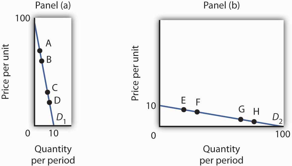
The table gives the prices and quantities corresponding to each of the points shown on the two demand curves.
Demand curve D1 [Panel (a)] Demand curve D2 [Panel (b)] Price Quantity Price Quantity A 80 2 E 8 20 B 70 3 F 7 30 C 30 7 G 3 70 D 20 8 H 2 80 - Compute the price elasticity of demand between points A and B and between points C and D on demand curve D1 in Panel (a). Are your results consistent with the notion that a linear demand curve is price elastic in its upper half and price inelastic in its lower half?
- Compute the price elasticity of demand between points E and F and between points G and H on demand curve D2 in Panel (b). Are your results consistent with the notion that a linear demand curve is price elastic in its upper half and price inelastic in its lower half?
- Compare total spending at points A and B on D1 in Panel (a). Is your result consistent with your finding about the price elasticity of demand between those two points?
- Compare total spending at points C and D on D1 in Panel (a). Is your result consistent with your finding about the price elasticity of demand between those two points?
- Compare total spending at points E and F on D2 in Panel (b). Is your result consistent with your finding about the price elasticity of demand between those two points?
- Compare total spending at points G and H on D2 in Panel (b). Is your result consistent with your finding about the price elasticity of demand between those two points?
-
Suppose Janice buys the following amounts of various food items depending on her weekly income:
Weekly Income Hamburgers Pizza Ice Cream Sundaes $500 3 3 2 $750 4 2 2 - Compute Janice’s income elasticity of demand for hamburgers.
- Compute Janice’s income elasticity of demand for pizza.
- Compute Janice’s income elasticity of demand for ice cream sundaes.
- Classify each good as normal or inferior.
-
Suppose the following table describes Jocelyn’s weekly snack purchases, which vary depending on the price of a bag of chips:
Price of bag of chips Bags of chips Containers of salsa Bags of pretzels Cans of soda $1.00 2 3 1 4 $1.50 1 2 2 4 - Compute the cross price elasticity of salsa with respect to the price of a bag of chips.
- Compute the cross price elasticity of pretzels with respect to the price of a bag of chips.
- Compute the cross price elasticity of soda with respect to the price of a bag of chips.
- Are chips and salsa substitutes or complements? How do you know?
- Are chips and pretzels substitutes or complements? How do you know?
- Are chips and soda substitutes or complements? How do you know?
-
The table below describes the supply curve for light bulbs:
Price per light bulb Quantity supplied per day $1.00 500 1.50 3,000 2.00 4,000 2.50 4,500 3.00 4,500 Compute the price elasticity of supply and determine whether supply is price elastic, price inelastic, perfectly elastic, perfectly inelastic, or unit elastic:
- when the price of a light bulb increases from $1.00 to $1.50.
- when the price of a light bulb increases from $1.50 to $2.00.
- when the price of a light bulb increases from $2.00 to $2.50.
- when the price of a light bulb increases from $2.50 to $3.00.