This is “The Coefficient of Determination”, section 10.6 from the book Beginning Statistics (v. 1.0). For details on it (including licensing), click here.
For more information on the source of this book, or why it is available for free, please see the project's home page. You can browse or download additional books there. To download a .zip file containing this book to use offline, simply click here.


10.6 The Coefficient of Determination
Learning Objective
- To learn what the coefficient of determination is, how to compute it, and what it tells us about the relationship between two variables x and y.
If the scatter diagram of a set of pairs shows neither an upward or downward trend, then the horizontal line fits it well, as illustrated in Figure 10.11. The lack of any upward or downward trend means that when an element of the population is selected at random, knowing the value of the measurement x for that element is not helpful in predicting the value of the measurement y.
Figure 10.11
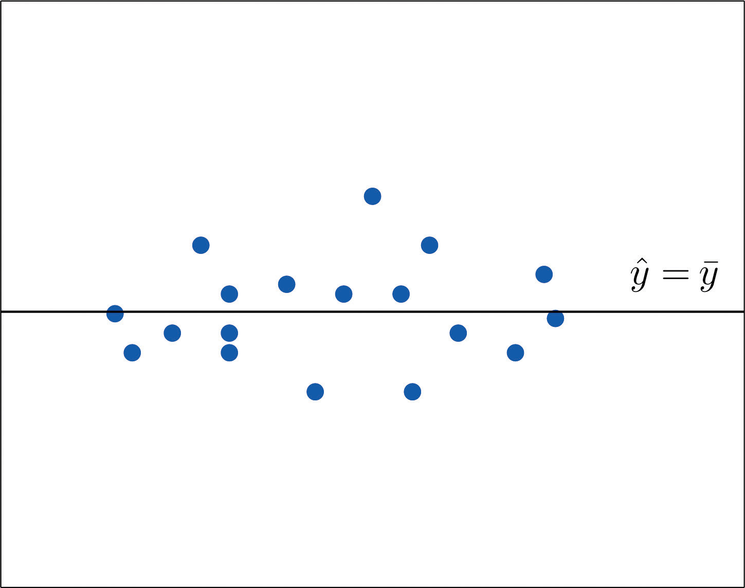
The line fits the scatter diagram well.
If the scatter diagram shows a linear trend upward or downward then it is useful to compute the least squares regression line and use it in predicting y. Figure 10.12 "Same Scatter Diagram with Two Approximating Lines" illustrates this. In each panel we have plotted the height and weight data of Section 10.1 "Linear Relationships Between Variables". This is the same scatter plot as Figure 10.2 "Plot of Height and Weight Pairs", with the average value line superimposed on it in the left panel and the least squares regression line imposed on it in the right panel. The errors are indicated graphically by the vertical line segments.
Figure 10.12 Same Scatter Diagram with Two Approximating Lines
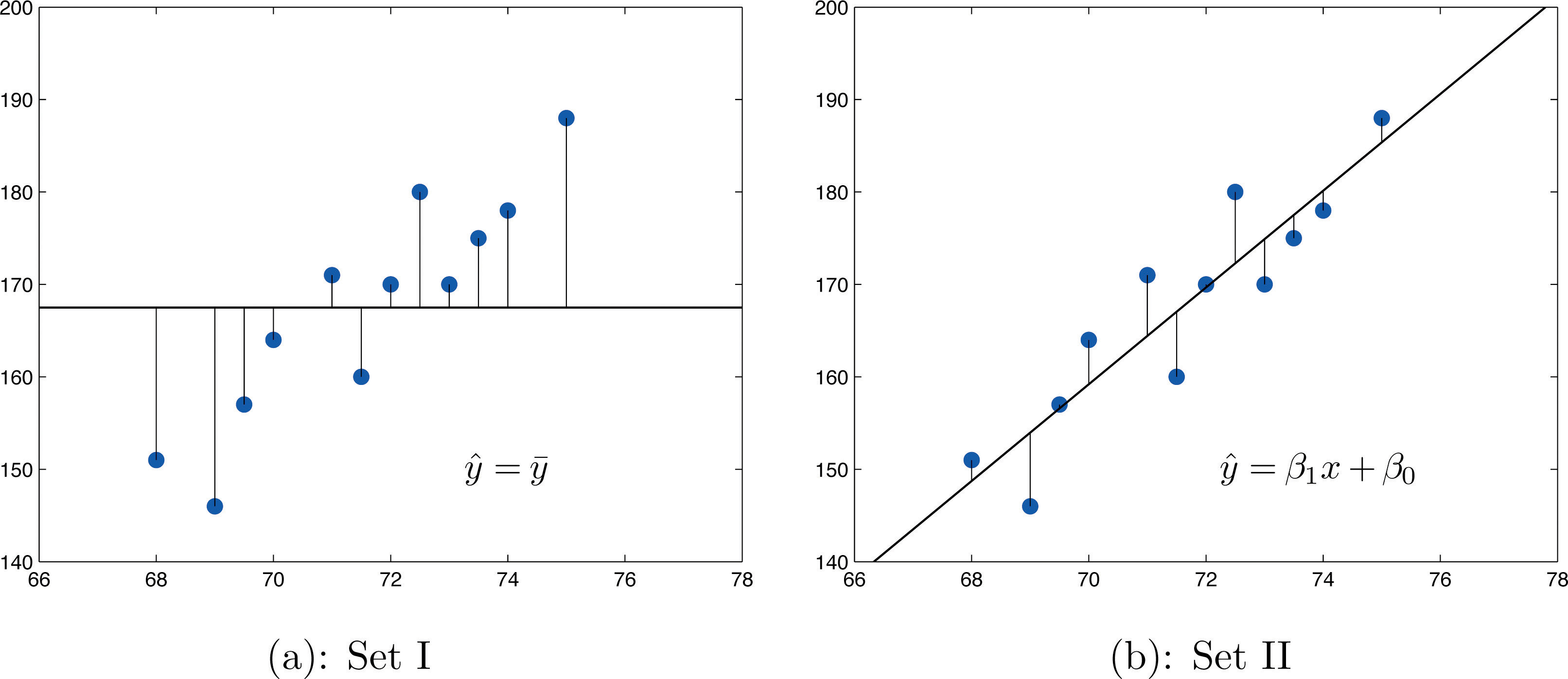
The sum of the squared errors computed for the regression line, , is smaller than the sum of the squared errors computed for any other line. In particular it is less than the sum of the squared errors computed using the line , which sum is actually the number that we have seen several times already. A measure of how useful it is to use the regression equation for prediction of y is how much smaller is than In particular, the proportion of the sum of the squared errors for the line that is eliminated by going over to the least squares regression line is
We can think of as the proportion of the variability in y that cannot be accounted for by the linear relationship between x and y, since it is still there even when x is taken into account in the best way possible (using the least squares regression line; remember that is the smallest the sum of the squared errors can be for any line). Seen in this light, the coefficient of determination, the complementary proportion of the variability in y, is the proportion of the variability in all the y measurements that is accounted for by the linear relationship between x and y.
In the context of linear regression the coefficient of determination is always the square of the correlation coefficient r discussed in Section 10.2 "The Linear Correlation Coefficient". Thus the coefficient of determination is denoted r2, and we have two additional formulas for computing it.
Definition
The coefficient of determinationA number that measures the proportion of the variability in y that is explained by x. of a collection of pairs is the number r2 computed by any of the following three expressions:
It measures the proportion of the variability in y that is accounted for by the linear relationship between x and y.
If the correlation coefficient r is already known then the coefficient of determination can be computed simply by squaring r, as the notation indicates,
Example 10
The value of used vehicles of the make and model discussed in Note 10.19 "Example 3" in Section 10.4 "The Least Squares Regression Line" varies widely. The most expensive automobile in the sample in Table 10.3 "Data on Age and Value of Used Automobiles of a Specific Make and Model" has value $30,500, which is nearly half again as much as the least expensive one, which is worth $20,400. Find the proportion of the variability in value that is accounted for by the linear relationship between age and value.
Solution:
The proportion of the variability in value y that is accounted for by the linear relationship between it and age x is given by the coefficient of determination, r2. Since the correlation coefficient r was already computed in Note 10.19 "Example 3" as , About 67% of the variability in the value of this vehicle can be explained by its age.
Example 11
Use each of the three formulas for the coefficient of determination to compute its value for the example of ages and values of vehicles.
Solution:
In Note 10.19 "Example 3" in Section 10.4 "The Least Squares Regression Line" we computed the exact values
In Note 10.24 "Example 5" in Section 10.4 "The Least Squares Regression Line" we computed the exact value
Inserting these values into the formulas in the definition, one after the other, gives
which rounds to 0.670. The discrepancy between the value here and in the previous example is because a rounded value of r from Note 10.19 "Example 3" was used there. The actual value of r before rounding is 0.8186864772, which when squared gives the value for r2 obtained here.
The coefficient of determination r2 can always be computed by squaring the correlation coefficient r if it is known. Any one of the defining formulas can also be used. Typically one would make the choice based on which quantities have already been computed. What should be avoided is trying to compute r by taking the square root of r2, if it is already known, since it is easy to make a sign error this way. To see what can go wrong, suppose Taking the square root of a positive number with any calculating device will always return a positive result. The square root of 0.64 is 0.8. However, the actual value of r might be the negative number −0.8.
Key Takeaways
- The coefficient of determination r2 estimates the proportion of the variability in the variable y that is explained by the linear relationship between y and the variable x.
- There are several formulas for computing r2. The choice of which one to use can be based on which quantities have already been computed so far.
Exercises
-
For the sample data set of Exercise 1 of Section 10.2 "The Linear Correlation Coefficient" find the coefficient of determination using the formula Confirm your answer by squaring r as computed in that exercise.
-
For the sample data set of Exercise 2 of Section 10.2 "The Linear Correlation Coefficient" find the coefficient of determination using the formula Confirm your answer by squaring r as computed in that exercise.
-
For the sample data set of Exercise 3 of Section 10.2 "The Linear Correlation Coefficient" find the coefficient of determination using the formula Confirm your answer by squaring r as computed in that exercise.
-
For the sample data set of Exercise 4 of Section 10.2 "The Linear Correlation Coefficient" find the coefficient of determination using the formula Confirm your answer by squaring r as computed in that exercise.
-
For the sample data set of Exercise 5 of Section 10.2 "The Linear Correlation Coefficient" find the coefficient of determination using the formula Confirm your answer by squaring r as computed in that exercise.
-
For the sample data set of Exercise 6 of Section 10.2 "The Linear Correlation Coefficient" find the coefficient of determination using the formula Confirm your answer by squaring r as computed in that exercise.
-
For the sample data set of Exercise 7 of Section 10.2 "The Linear Correlation Coefficient" find the coefficient of determination using the formula Confirm your answer by squaring r as computed in that exercise.
-
For the sample data set of Exercise 8 of Section 10.2 "The Linear Correlation Coefficient" find the coefficient of determination using the formula Confirm your answer by squaring r as computed in that exercise.
-
For the sample data set of Exercise 9 of Section 10.2 "The Linear Correlation Coefficient" find the coefficient of determination using the formula Confirm your answer by squaring r as computed in that exercise.
-
For the sample data set of Exercise 9 of Section 10.2 "The Linear Correlation Coefficient" find the coefficient of determination using the formula Confirm your answer by squaring r as computed in that exercise.
Basic
For the Basic and Application exercises in this section use the computations that were done for the exercises with the same number in Section 10.2 "The Linear Correlation Coefficient", Section 10.4 "The Least Squares Regression Line", and Section 10.5 "Statistical Inferences About ".
-
For the data in Exercise 11 of Section 10.2 "The Linear Correlation Coefficient" compute the coefficient of determination and interpret its value in the context of age and vocabulary.
-
For the data in Exercise 12 of Section 10.2 "The Linear Correlation Coefficient" compute the coefficient of determination and interpret its value in the context of vehicle weight and braking distance.
-
For the data in Exercise 13 of Section 10.2 "The Linear Correlation Coefficient" compute the coefficient of determination and interpret its value in the context of age and resting heart rate. In the age range of the data, does age seem to be a very important factor with regard to heart rate?
-
For the data in Exercise 14 of Section 10.2 "The Linear Correlation Coefficient" compute the coefficient of determination and interpret its value in the context of wind speed and wave height. Does wind speed seem to be a very important factor with regard to wave height?
-
For the data in Exercise 15 of Section 10.2 "The Linear Correlation Coefficient" find the proportion of the variability in revenue that is explained by level of advertising.
-
For the data in Exercise 16 of Section 10.2 "The Linear Correlation Coefficient" find the proportion of the variability in adult height that is explained by the variation in length at age two.
-
For the data in Exercise 17 of Section 10.2 "The Linear Correlation Coefficient" compute the coefficient of determination and interpret its value in the context of course average before the final exam and score on the final exam.
-
For the data in Exercise 18 of Section 10.2 "The Linear Correlation Coefficient" compute the coefficient of determination and interpret its value in the context of acres planted and acres harvested.
-
For the data in Exercise 19 of Section 10.2 "The Linear Correlation Coefficient" compute the coefficient of determination and interpret its value in the context of the amount of the medication consumed and blood concentration of the active ingredient.
-
For the data in Exercise 20 of Section 10.2 "The Linear Correlation Coefficient" compute the coefficient of determination and interpret its value in the context of tree size and age.
-
For the data in Exercise 21 of Section 10.2 "The Linear Correlation Coefficient" find the proportion of the variability in 28-day strength of concrete that is accounted for by variation in 3-day strength.
-
For the data in Exercise 22 of Section 10.2 "The Linear Correlation Coefficient" find the proportion of the variability in energy demand that is accounted for by variation in average temperature.
Applications
-
Large Data Set 1 lists the SAT scores and GPAs of 1,000 students. Compute the coefficient of determination and interpret its value in the context of SAT scores and GPAs.
-
Large Data Set 12 lists the golf scores on one round of golf for 75 golfers first using their own original clubs, then using clubs of a new, experimental design (after two months of familiarization with the new clubs). Compute the coefficient of determination and interpret its value in the context of golf scores with the two kinds of golf clubs.
http://www.flatworldknowledge.com/sites/all/files/data12.xls
-
Large Data Set 13 records the number of bidders and sales price of a particular type of antique grandfather clock at 60 auctions. Compute the coefficient of determination and interpret its value in the context of the number of bidders at an auction and the price of this type of antique grandfather clock.
http://www.flatworldknowledge.com/sites/all/files/data13.xls
Large Data Set Exercises
Answers
-
0.848
-
-
0.631
-
-
0.5
-
-
0.766
-
-
0.715
-
-
0.898; about 90% of the variability in vocabulary is explained by age
-
-
0.503; about 50% of the variability in heart rate is explained by age. Age is a significant but not dominant factor in explaining heart rate.
-
-
The proportion is r2 = 0.692.
-
-
0.563; about 56% of the variability in final exam scores is explained by course average before the final exam
-
-
0.931; about 93% of the variability in the blood concentration of the active ingredient is explained by the amount of the medication consumed
-
-
The proportion is r2 = 0.984.
-