This is “The Least Squares Regression Line”, section 10.4 from the book Beginning Statistics (v. 1.0). For details on it (including licensing), click here.
For more information on the source of this book, or why it is available for free, please see the project's home page. You can browse or download additional books there. To download a .zip file containing this book to use offline, simply click here.


10.4 The Least Squares Regression Line
Learning Objectives
- To learn how to measure how well a straight line fits a collection of data.
- To learn how to construct the least squares regression line, the straight line that best fits a collection of data.
- To learn the meaning of the slope of the least squares regression line.
- To learn how to use the least squares regression line to estimate the response variable y in terms of the predictor variable x.
Goodness of Fit of a Straight Line to Data
Once the scatter diagram of the data has been drawn and the model assumptions described in the previous sections at least visually verified (and perhaps the correlation coefficient r computed to quantitatively verify the linear trend), the next step in the analysis is to find the straight line that best fits the data. We will explain how to measure how well a straight line fits a collection of points by examining how well the line fits the data set
(which will be used as a running example for the next three sections). We will write the equation of this line as with an accent on the y to indicate that the y-values computed using this equation are not from the data. We will do this with all lines approximating data sets. The line was selected as one that seems to fit the data reasonably well.
The idea for measuring the goodness of fit of a straight line to data is illustrated in Figure 10.6 "Plot of the Five-Point Data and the Line ", in which the graph of the line has been superimposed on the scatter plot for the sample data set.
Figure 10.6 Plot of the Five-Point Data and the Line
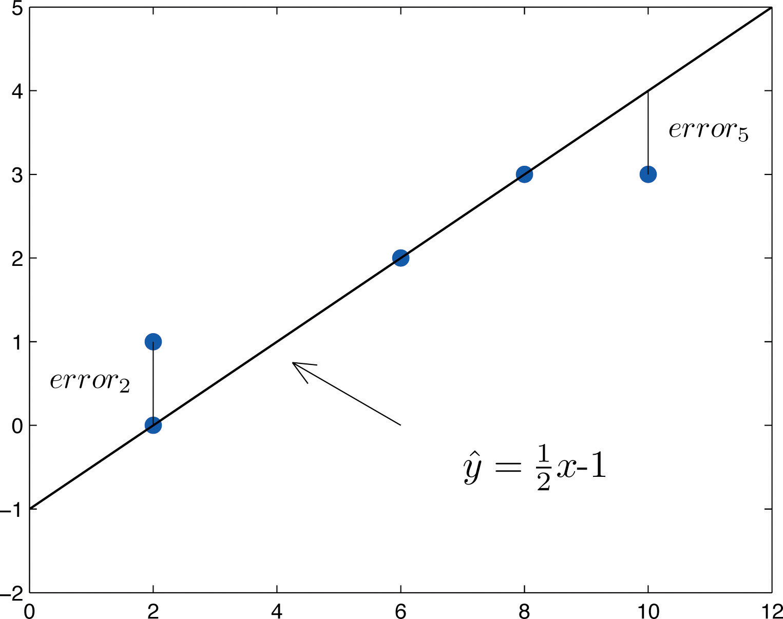
To each point in the data set there is associated an “errorUsing , the actual y-value of a data point minus the y-value that is computed from the equation of the line fitting the data.,” the positive or negative vertical distance from the point to the line: positive if the point is above the line and negative if it is below the line. The error can be computed as the actual y-value of the point minus the y-value that is “predicted” by inserting the x-value of the data point into the formula for the line:
The computation of the error for each of the five points in the data set is shown in Table 10.1 "The Errors in Fitting Data with a Straight Line".
Table 10.1 The Errors in Fitting Data with a Straight Line
| x | y | ||||
|---|---|---|---|---|---|
| 2 | 0 | 0 | 0 | 0 | |
| 2 | 1 | 0 | 1 | 1 | |
| 6 | 2 | 2 | 0 | 0 | |
| 8 | 3 | 3 | 0 | 0 | |
| 10 | 3 | 4 | −1 | 1 | |
| Σ | - | - | - | 0 | 2 |
A first thought for a measure of the goodness of fit of the line to the data would be simply to add the errors at every point, but the example shows that this cannot work well in general. The line does not fit the data perfectly (no line can), yet because of cancellation of positive and negative errors the sum of the errors (the fourth column of numbers) is zero. Instead goodness of fit is measured by the sum of the squares of the errors. Squaring eliminates the minus signs, so no cancellation can occur. For the data and line in Figure 10.6 "Plot of the Five-Point Data and the Line " the sum of the squared errors (the last column of numbers) is 2. This number measures the goodness of fit of the line to the data.
Definition
The goodness of fit of a line to a set of n pairs of numbers in a sample is the sum of the squared errors
(n terms in the sum, one for each data pair).
The Least Squares Regression Line
Given any collection of pairs of numbers (except when all the x-values are the same) and the corresponding scatter diagram, there always exists exactly one straight line that fits the data better than any other, in the sense of minimizing the sum of the squared errors. It is called the least squares regression line. Moreover there are formulas for its slope and y-intercept.
Definition
Given a collection of pairs of numbers (in which not all the x-values are the same), there is a line that best fits the data in the sense of minimizing the sum of the squared errors. It is called the least squares regression lineThe line that best fits a set of sample data in the sense of minimizing the sum of the squared errors.. Its slope and y-intercept are computed using the formulas
where
is the mean of all the x-values, is the mean of all the y-values, and n is the number of pairs in the data set.
The equation specifying the least squares regression line is called the least squares regression equationThe equation of the least squares regression line..
Remember from Section 10.3 "Modelling Linear Relationships with Randomness Present" that the line with the equation is called the population regression line. The numbers and are statistics that estimate the population parameters and
We will compute the least squares regression line for the five-point data set, then for a more practical example that will be another running example for the introduction of new concepts in this and the next three sections.
Example 2
Find the least squares regression line for the five-point data set
and verify that it fits the data better than the line considered in Section 10.4.1 "Goodness of Fit of a Straight Line to Data".
Solution:
In actual practice computation of the regression line is done using a statistical computation package. In order to clarify the meaning of the formulas we display the computations in tabular form.
| x | y | x2 | ||
|---|---|---|---|---|
| 2 | 0 | 4 | 0 | |
| 2 | 1 | 4 | 2 | |
| 6 | 2 | 36 | 12 | |
| 8 | 3 | 64 | 24 | |
| 10 | 3 | 100 | 30 | |
| Σ | 28 | 9 | 208 | 68 |
In the last line of the table we have the sum of the numbers in each column. Using them we compute:
so that
The least squares regression line for these data is
The computations for measuring how well it fits the sample data are given in Table 10.2 "The Errors in Fitting Data with the Least Squares Regression Line". The sum of the squared errors is the sum of the numbers in the last column, which is 0.75. It is less than 2, the sum of the squared errors for the fit of the line to this data set.
Table 10.2 The Errors in Fitting Data with the Least Squares Regression Line
| x | y | |||
|---|---|---|---|---|
| 2 | 0 | 0.5625 | −0.5625 | 0.31640625 |
| 2 | 1 | 0.5625 | 0.4375 | 0.19140625 |
| 6 | 2 | 1.9375 | 0.0625 | 0.00390625 |
| 8 | 3 | 2.6250 | 0.3750 | 0.14062500 |
| 10 | 3 | 3.3125 | −0.3125 | 0.09765625 |
Example 3
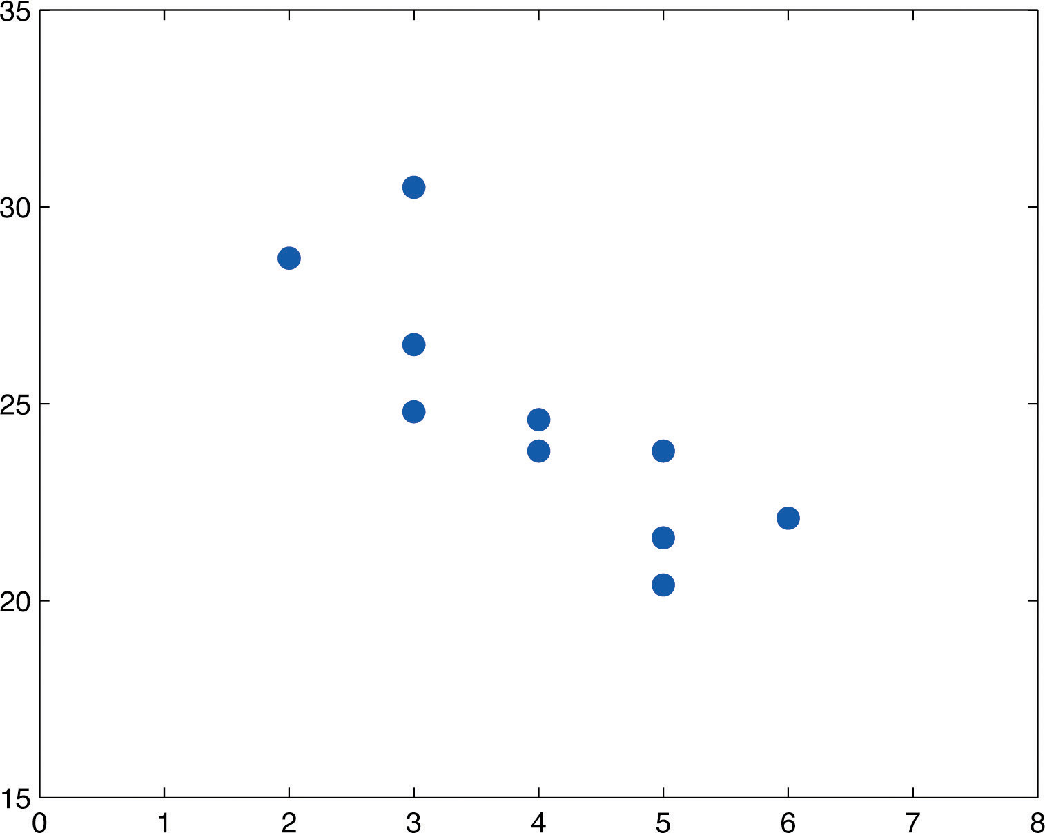
Table 10.3 "Data on Age and Value of Used Automobiles of a Specific Make and Model" shows the age in years and the retail value in thousands of dollars of a random sample of ten automobiles of the same make and model.
- Construct the scatter diagram.
- Compute the linear correlation coefficient r. Interpret its value in the context of the problem.
- Compute the least squares regression line. Plot it on the scatter diagram.
- Interpret the meaning of the slope of the least squares regression line in the context of the problem.
- Suppose a four-year-old automobile of this make and model is selected at random. Use the regression equation to predict its retail value.
- Suppose a 20-year-old automobile of this make and model is selected at random. Use the regression equation to predict its retail value. Interpret the result.
- Comment on the validity of using the regression equation to predict the price of a brand new automobile of this make and model.
Table 10.3 Data on Age and Value of Used Automobiles of a Specific Make and Model
| x | 2 | 3 | 3 | 3 | 4 | 4 | 5 | 5 | 5 | 6 |
| y | 28.7 | 24.8 | 26.0 | 30.5 | 23.8 | 24.6 | 23.8 | 20.4 | 21.6 | 22.1 |
Solution:
- The scatter diagram is shown in Figure 10.7 "Scatter Diagram for Age and Value of Used Automobiles".
Figure 10.7 Scatter Diagram for Age and Value of Used Automobiles
-
We must first compute , , , which means computing , , , , and Using a computing device we obtain
Thus
so that
The age and value of this make and model automobile are moderately strongly negatively correlated. As the age increases, the value of the automobile tends to decrease.
-
Using the values of and computed in part (b),
Thus using the values of and from part (b),
The equation of the least squares regression line for these sample data is
Figure 10.8 "Scatter Diagram and Regression Line for Age and Value of Used Automobiles" shows the scatter diagram with the graph of the least squares regression line superimposed.
Figure 10.8 Scatter Diagram and Regression Line for Age and Value of Used Automobiles
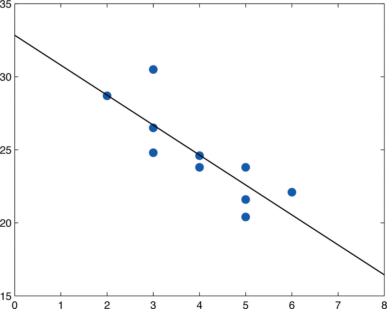
- The slope −2.05 means that for each unit increase in x (additional year of age) the average value of this make and model vehicle decreases by about 2.05 units (about $2,050).
-
Since we know nothing about the automobile other than its age, we assume that it is of about average value and use the average value of all four-year-old vehicles of this make and model as our estimate. The average value is simply the value of obtained when the number 4 is inserted for x in the least squares regression equation:
which corresponds to $24,630.
-
Now we insert into the least squares regression equation, to obtain
which corresponds to −$8,170. Something is wrong here, since a negative makes no sense. The error arose from applying the regression equation to a value of x not in the range of x-values in the original data, from two to six years.
Applying the regression equation to a value of x outside the range of x-values in the data set is called extrapolation. It is an invalid use of the regression equation and should be avoided.
- The price of a brand new vehicle of this make and model is the value of the automobile at age 0. If the value is inserted into the regression equation the result is always , the y-intercept, in this case 32.83, which corresponds to $32,830. But this is a case of extrapolation, just as part (f) was, hence this result is invalid, although not obviously so. In the context of the problem, since automobiles tend to lose value much more quickly immediately after they are purchased than they do after they are several years old, the number $32,830 is probably an underestimate of the price of a new automobile of this make and model.
For emphasis we highlight the points raised by parts (f) and (g) of the example.
Definition
The process of using the least squares regression equation to estimate the value of y at a value of x that does not lie in the range of the x-values in the data set that was used to form the regression line is called extrapolationThe process of using the least squares regression equation to estimate the value of y at an x value not in the proper range.. It is an invalid use of the regression equation that can lead to errors, hence should be avoided.
The Sum of the Squared Errors
In general, in order to measure the goodness of fit of a line to a set of data, we must compute the predicted y-value at every point in the data set, compute each error, square it, and then add up all the squares. In the case of the least squares regression line, however, the line that best fits the data, the sum of the squared errors can be computed directly from the data using the following formula.
The sum of the squared errors for the least squares regression line is denoted by It can be computed using the formula
Example 4
Find the sum of the squared errors for the least squares regression line for the five-point data set
Do so in two ways:
- using the definition ;
- using the formula
Solution:
- The least squares regression line was computed in Note 10.18 "Example 2" and is was found at the end of that example using the definition The computations were tabulated in Table 10.2 "The Errors in Fitting Data with the Least Squares Regression Line". is the sum of the numbers in the last column, which is 0.75.
-
The numbers and were already computed in Note 10.18 "Example 2" in the process of finding the least squares regression line. So was the number We must compute To do so it is necessary to first compute Then
so that
Example 5
Find the sum of the squared errors for the least squares regression line for the data set, presented in Table 10.3 "Data on Age and Value of Used Automobiles of a Specific Make and Model", on age and values of used vehicles in Note 10.19 "Example 3".
Solution:
From Note 10.19 "Example 3" we already know that
To compute we first compute
Then
Therefore
Key Takeaways
- How well a straight line fits a data set is measured by the sum of the squared errors.
- The least squares regression line is the line that best fits the data. Its slope and y-intercept are computed from the data using formulas.
- The slope of the least squares regression line estimates the size and direction of the mean change in the dependent variable y when the independent variable x is increased by one unit.
- The sum of the squared errors of the least squares regression line can be computed using a formula, without having to compute all the individual errors.
Exercises
-
Compute the least squares regression line for the data in Exercise 1 of Section 10.2 "The Linear Correlation Coefficient".
-
Compute the least squares regression line for the data in Exercise 2 of Section 10.2 "The Linear Correlation Coefficient".
-
Compute the least squares regression line for the data in Exercise 3 of Section 10.2 "The Linear Correlation Coefficient".
-
Compute the least squares regression line for the data in Exercise 4 of Section 10.2 "The Linear Correlation Coefficient".
-
For the data in Exercise 5 of Section 10.2 "The Linear Correlation Coefficient"
- Compute the least squares regression line.
- Compute the sum of the squared errors using the definition
- Compute the sum of the squared errors using the formula
-
For the data in Exercise 6 of Section 10.2 "The Linear Correlation Coefficient"
- Compute the least squares regression line.
- Compute the sum of the squared errors using the definition
- Compute the sum of the squared errors using the formula
-
Compute the least squares regression line for the data in Exercise 7 of Section 10.2 "The Linear Correlation Coefficient".
-
Compute the least squares regression line for the data in Exercise 8 of Section 10.2 "The Linear Correlation Coefficient".
-
For the data in Exercise 9 of Section 10.2 "The Linear Correlation Coefficient"
- Compute the least squares regression line.
- Can you compute the sum of the squared errors using the definition ? Explain.
- Compute the sum of the squared errors using the formula
-
For the data in Exercise 10 of Section 10.2 "The Linear Correlation Coefficient"
- Compute the least squares regression line.
- Can you compute the sum of the squared errors using the definition ? Explain.
- Compute the sum of the squared errors using the formula
Basic
For the Basic and Application exercises in this section use the computations that were done for the exercises with the same number in Section 10.2 "The Linear Correlation Coefficient".
-
For the data in Exercise 11 of Section 10.2 "The Linear Correlation Coefficient"
- Compute the least squares regression line.
- On average, how many new words does a child from 13 to 18 months old learn each month? Explain.
- Estimate the average vocabulary of all 16-month-old children.
-
For the data in Exercise 12 of Section 10.2 "The Linear Correlation Coefficient"
- Compute the least squares regression line.
- On average, how many additional feet are added to the braking distance for each additional 100 pounds of weight? Explain.
- Estimate the average braking distance of all cars weighing 3,000 pounds.
-
For the data in Exercise 13 of Section 10.2 "The Linear Correlation Coefficient"
- Compute the least squares regression line.
- Estimate the average resting heart rate of all 40-year-old men.
- Estimate the average resting heart rate of all newborn baby boys. Comment on the validity of the estimate.
-
For the data in Exercise 14 of Section 10.2 "The Linear Correlation Coefficient"
- Compute the least squares regression line.
- Estimate the average wave height when the wind is blowing at 10 miles per hour.
- Estimate the average wave height when there is no wind blowing. Comment on the validity of the estimate.
-
For the data in Exercise 15 of Section 10.2 "The Linear Correlation Coefficient"
- Compute the least squares regression line.
- On average, for each additional thousand dollars spent on advertising, how does revenue change? Explain.
- Estimate the revenue if $2,500 is spent on advertising next year.
-
For the data in Exercise 16 of Section 10.2 "The Linear Correlation Coefficient"
- Compute the least squares regression line.
- On average, for each additional inch of height of two-year-old girl, what is the change in the adult height? Explain.
- Predict the adult height of a two-year-old girl who is 33 inches tall.
-
For the data in Exercise 17 of Section 10.2 "The Linear Correlation Coefficient"
- Compute the least squares regression line.
- Compute using the formula
- Estimate the average final exam score of all students whose course average just before the exam is 85.
-
For the data in Exercise 18 of Section 10.2 "The Linear Correlation Coefficient"
- Compute the least squares regression line.
- Compute using the formula
- Estimate the number of acres that would be harvested if 90 million acres of corn were planted.
-
For the data in Exercise 19 of Section 10.2 "The Linear Correlation Coefficient"
- Compute the least squares regression line.
- Interpret the value of the slope of the least squares regression line in the context of the problem.
- Estimate the average concentration of the active ingredient in the blood in men after consuming 1 ounce of the medication.
-
For the data in Exercise 20 of Section 10.2 "The Linear Correlation Coefficient"
- Compute the least squares regression line.
- Interpret the value of the slope of the least squares regression line in the context of the problem.
- Estimate the age of an oak tree whose girth five feet off the ground is 92 inches.
-
For the data in Exercise 21 of Section 10.2 "The Linear Correlation Coefficient"
- Compute the least squares regression line.
- The 28-day strength of concrete used on a certain job must be at least 3,200 psi. If the 3-day strength is 1,300 psi, would we anticipate that the concrete will be sufficiently strong on the 28th day? Explain fully.
-
For the data in Exercise 22 of Section 10.2 "The Linear Correlation Coefficient"
- Compute the least squares regression line.
- If the power facility is called upon to provide more than 95 million watt-hours tomorrow then energy will have to be purchased from elsewhere at a premium. The forecast is for an average temperature of 42 degrees. Should the company plan on purchasing power at a premium?
Applications
-
Verify that no matter what the data are, the least squares regression line always passes through the point with coordinates Hint: Find the predicted value of y when
-
In Exercise 1 you computed the least squares regression line for the data in Exercise 1 of Section 10.2 "The Linear Correlation Coefficient".
-
Reverse the roles of x and y and compute the least squares regression line for the new data set
- Interchanging x and y corresponds geometrically to reflecting the scatter plot in a 45-degree line. Reflecting the regression line for the original data the same way gives a line with the equation Is this the equation that you got in part (a)? Can you figure out why not? Hint: Think about how x and y are treated differently geometrically in the computation of the goodness of fit.
- Compute for each line and see if they fit the same, or if one fits the data better than the other.
-
Additional Exercises
-
Large Data Set 1 lists the SAT scores and GPAs of 1,000 students.
http://www.flatworldknowledge.com/sites/all/files/data1.xls
- Compute the least squares regression line with SAT score as the independent variable (x) and GPA as the dependent variable (y).
- Interpret the meaning of the slope of regression line in the context of problem.
- Compute , the measure of the goodness of fit of the regression line to the sample data.
- Estimate the GPA of a student whose SAT score is 1350.
-
Large Data Set 12 lists the golf scores on one round of golf for 75 golfers first using their own original clubs, then using clubs of a new, experimental design (after two months of familiarization with the new clubs).
http://www.flatworldknowledge.com/sites/all/files/data12.xls
- Compute the least squares regression line with scores using the original clubs as the independent variable (x) and scores using the new clubs as the dependent variable (y).
- Interpret the meaning of the slope of regression line in the context of problem.
- Compute , the measure of the goodness of fit of the regression line to the sample data.
- Estimate the score with the new clubs of a golfer whose score with the old clubs is 73.
-
Large Data Set 13 records the number of bidders and sales price of a particular type of antique grandfather clock at 60 auctions.
http://www.flatworldknowledge.com/sites/all/files/data13.xls
- Compute the least squares regression line with the number of bidders present at the auction as the independent variable (x) and sales price as the dependent variable (y).
- Interpret the meaning of the slope of regression line in the context of problem.
- Compute , the measure of the goodness of fit of the regression line to the sample data.
- Estimate the sales price of a clock at an auction at which the number of bidders is seven.
Large Data Set Exercises
Answers
-
-
-
-
-
,
-
-
-
-
, (cannot use the definition to compute)
-
-
- ,
- 4.8,
- 21.6
-
-
- ,
- 73.8,
- 69.2, invalid extrapolation
-
-
- ,
- increases by $42,024,
- $224,562
-
-
- ,
- 2151.93367,
- 80.3
-
-
- ,
- For each additional ounce of medication consumed blood concentration of the active ingredient increases by 0.043 %,
- 0.044%
-
-
- ,
- Predicted 28-day strength is 3,514 psi; sufficiently strong
-
-
- On average, every 100 point increase in SAT score adds 0.16 point to the GPA.
-
-
- On average, every 1 additional bidder at an auction raises the price by 116.62 dollars.