This is “Two-Sample Problems”, chapter 9 from the book Beginning Statistics (v. 1.0). For details on it (including licensing), click here.
For more information on the source of this book, or why it is available for free, please see the project's home page. You can browse or download additional books there. To download a .zip file containing this book to use offline, simply click here.


Chapter 9 Two-Sample Problems
The previous two chapters treated the questions of estimating and making inferences about a parameter of a single population. In this chapter we consider a comparison of parameters that belong to two different populations. For example, we might wish to compare the average income of all adults in one region of the country with the average income of those in another region, or we might wish to compare the proportion of all men who are vegetarians with the proportion of all women who are vegetarians.
We will study construction of confidence intervals and tests of hypotheses in four situations, depending on the parameter of interest, the sizes of the samples drawn from each of the populations, and the method of sampling. We also examine sample size considerations.
9.1 Comparison of Two Population Means: Large, Independent Samples
Learning Objectives
- To understand the logical framework for estimating the difference between the means of two distinct populations and performing tests of hypotheses concerning those means.
- To learn how to construct a confidence interval for the difference in the means of two distinct populations using large, independent samples.
- To learn how to perform a test of hypotheses concerning the difference between the means of two distinct populations using large, independent samples.
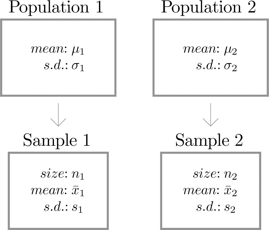
Suppose we wish to compare the means of two distinct populations. Figure 9.1 "Independent Sampling from Two Populations" illustrates the conceptual framework of our investigation in this and the next section. Each population has a mean and a standard deviation. We arbitrarily label one population as Population 1 and the other as Population 2, and subscript the parameters with the numbers 1 and 2 to tell them apart. We draw a random sample from Population 1 and label the sample statistics it yields with the subscript 1. Without reference to the first sample we draw a sample from Population 2 and label its sample statistics with the subscript 2.
Figure 9.1 Independent Sampling from Two Populations
Definition
Samples from two distinct populations are independent if each one is drawn without reference to the other, and has no connection with the other.
Our goal is to use the information in the samples to estimate the difference in the means of the two populations and to make statistically valid inferences about it.
Confidence Intervals
Since the mean of the sample drawn from Population 1 is a good estimator of and the mean of the sample drawn from Population 2 is a good estimator of , a reasonable point estimate of the difference is In order to widen this point estimate into a confidence interval, we first suppose that both samples are large, that is, that both and If so, then the following formula for a confidence interval for is valid. The symbols and denote the squares of s1 and s2. (In the relatively rare case that both population standard deviations and are known they would be used instead of the sample standard deviations.)
Confidence Interval for the Difference Between Two Population Means: Large, Independent Samples
The samples must be independent, and each sample must be large: and
Example 1
To compare customer satisfaction levels of two competing cable television companies, 174 customers of Company 1 and 355 customers of Company 2 were randomly selected and were asked to rate their cable companies on a five-point scale, with 1 being least satisfied and 5 most satisfied. The survey results are summarized in the following table:
| Company 1 | Company 2 |
|---|---|
Construct a point estimate and a 99% confidence interval for , the difference in average satisfaction levels of customers of the two companies as measured on this five-point scale.
Solution:
The point estimate of is
In words, we estimate that the average customer satisfaction level for Company 1 is 0.27 points higher on this five-point scale than it is for Company 2.
To apply the formula for the confidence interval, proceed exactly as was done in Chapter 7 "Estimation". The 99% confidence level means that so that From Figure 12.3 "Critical Values of " we read directly that Thus
We are 99% confident that the difference in the population means lies in the interval , in the sense that in repeated sampling 99% of all intervals constructed from the sample data in this manner will contain In the context of the problem we say we are 99% confident that the average level of customer satisfaction for Company 1 is between 0.15 and 0.39 points higher, on this five-point scale, than that for Company 2.
Hypothesis Testing
Hypotheses concerning the relative sizes of the means of two populations are tested using the same critical value and p-value procedures that were used in the case of a single population. All that is needed is to know how to express the null and alternative hypotheses and to know the formula for the standardized test statistic and the distribution that it follows.
The null and alternative hypotheses will always be expressed in terms of the difference of the two population means. Thus the null hypothesis will always be written
where D0 is a number that is deduced from the statement of the situation. As was the case with a single population the alternative hypothesis can take one of the three forms, with the same terminology:
| Form of | Terminology |
|---|---|
| Left-tailed | |
| Right-tailed | |
| Two-tailed |
As long as the samples are independent and both are large the following formula for the standardized test statistic is valid, and it has the standard normal distribution. (In the relatively rare case that both population standard deviations and are known they would be used instead of the sample standard deviations.)
Standardized Test Statistic for Hypothesis Tests Concerning the Difference Between Two Population Means: Large, Independent Samples
The test statistic has the standard normal distribution.
The samples must be independent, and each sample must be large: and
Example 2
Refer to Note 9.4 "Example 1" concerning the mean satisfaction levels of customers of two competing cable television companies. Test at the 1% level of significance whether the data provide sufficient evidence to conclude that Company 1 has a higher mean satisfaction rating than does Company 2. Use the critical value approach.
Solution:
-
Step 1. If the mean satisfaction levels and are the same then , but we always express the null hypothesis in terms of the difference between and , hence H0 is To say that the mean customer satisfaction for Company 1 is higher than that for Company 2 means that , which in terms of their difference is The test is therefore
-
Step 2. Since the samples are independent and both are large the test statistic is
-
Step 3. Inserting the data into the formula for the test statistic gives
-
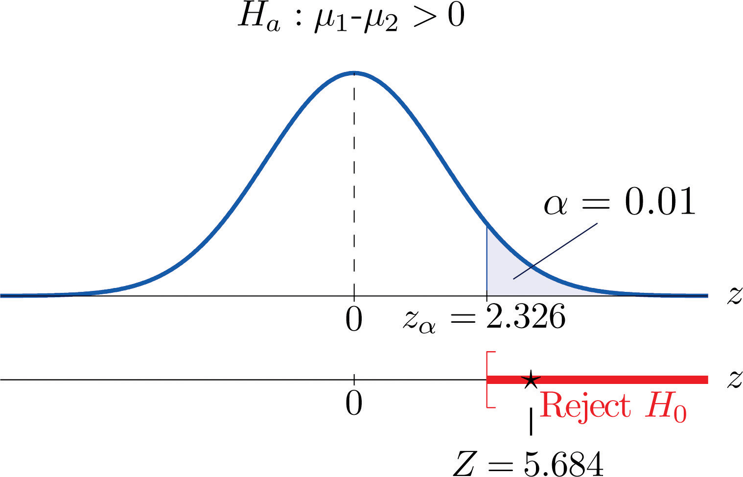
Step 4. Since the symbol in Ha is “>” this is a right-tailed test, so there is a single critical value, , which from the last line in Figure 12.3 "Critical Values of " we read off as 2.326. The rejection region is
Figure 9.2 Rejection Region and Test Statistic for Note 9.6 "Example 2"
-
Step 5. As shown in Figure 9.2 "Rejection Region and Test Statistic for " the test statistic falls in the rejection region. The decision is to reject H0. In the context of the problem our conclusion is:
The data provide sufficient evidence, at the 1% level of significance, to conclude that the mean customer satisfaction for Company 1 is higher than that for Company 2.
Example 3
Perform the test of Note 9.6 "Example 2" using the p-value approach.
Solution:
The first three steps are identical to those in Note 9.6 "Example 2".
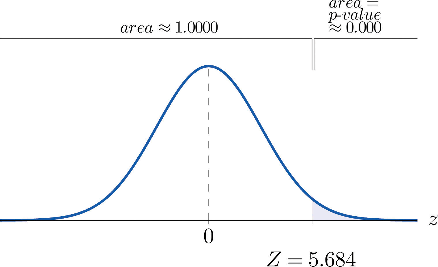
- Step 4. The observed significance or p-value of the test is the area of the right tail of the standard normal distribution that is cut off by the test statistic Z = 5.684. The number 5.684 is too large to appear in Figure 12.2 "Cumulative Normal Probability", which means that the area of the left tail that it cuts off is 1.0000 to four decimal places. The area that we seek, the area of the right tail, is therefore to four decimal places. See Figure 9.3. That is, to four decimal places. (The actual value is approximately )
Figure 9.3 P-Value for Note 9.7 "Example 3"
-
Step 5. Since 0.0000 < 0.01, so the decision is to reject the null hypothesis:
The data provide sufficient evidence, at the 1% level of significance, to conclude that the mean customer satisfaction for Company 1 is higher than that for Company 2.
Key Takeaways
- A point estimate for the difference in two population means is simply the difference in the corresponding sample means.
- In the context of estimating or testing hypotheses concerning two population means, “large” samples means that both samples are large.
- A confidence interval for the difference in two population means is computed using a formula in the same fashion as was done for a single population mean.
- The same five-step procedure used to test hypotheses concerning a single population mean is used to test hypotheses concerning the difference between two population means. The only difference is in the formula for the standardized test statistic.
Exercises
-
Construct the confidence interval for for the level of confidence and the data from independent samples given.
-
90% confidence,
, ,
, ,
-
99% confidence,
, ,
, ,
-
-
Construct the confidence interval for for the level of confidence and the data from independent samples given.
-
95% confidence,
, ,
, ,
-
90% confidence,
, ,
, ,
-
-
Construct the confidence interval for for the level of confidence and the data from independent samples given.
-
99.5% confidence,
, ,
, ,
-
95% confidence,
, ,
, ,
-
-
Construct the confidence interval for for the level of confidence and the data from independent samples given.
-
99.9% confidence,
, ,
, ,
-
90% confidence,
, ,
, ,
-
-
Perform the test of hypotheses indicated, using the data from independent samples given. Use the critical value approach. Compute the p-value of the test as well.
-
Test vs. @ ,
, ,
, ,
-
Test vs. @ ,
, ,
, ,
-
-
Perform the test of hypotheses indicated, using the data from independent samples given. Use the critical value approach. Compute the p-value of the test as well.
-
Test vs. @ ,
, ,
, ,
-
Test vs. @ ,
, ,
, ,
-
-
Perform the test of hypotheses indicated, using the data from independent samples given. Use the critical value approach. Compute the p-value of the test as well.
-
Test vs. @ ,
, ,
, ,
-
Test vs. @ ,
, ,
, ,
-
-
Perform the test of hypotheses indicated, using the data from independent samples given. Use the critical value approach. Compute the p-value of the test as well.
-
Test vs. @ ,
, ,
, ,
-
Test vs. @ ,
, ,
, ,
-
-
Perform the test of hypotheses indicated, using the data from independent samples given. Use the p-value approach.
-
Test vs. @ ,
, ,
, ,
-
Test vs. @ ,
, ,
, ,
-
-
Perform the test of hypotheses indicated, using the data from independent samples given. Use the p-value approach.
-
Test vs. @ ,
, ,
, ,
-
Test vs. @ ,
, ,
, ,
-
-
Perform the test of hypotheses indicated, using the data from independent samples given. Use the p-value approach.
-
Test vs. @ ,
, ,
, ,
-
Test vs. @ ,
, ,
, ,
-
-
Perform the test of hypotheses indicated, using the data from independent samples given. Use the p-value approach.
-
Test vs. @ ,
, ,
, ,
-
Test vs. @ ,
, ,
, ,
-
Basic
-
In order to investigate the relationship between mean job tenure in years among workers who have a bachelor’s degree or higher and those who do not, random samples of each type of worker were taken, with the following results.
n s Bachelor’s degree or higher 155 5.2 1.3 No degree 210 5.0 1.5 - Construct the 99% confidence interval for the difference in the population means based on these data.
- Test, at the 1% level of significance, the claim that mean job tenure among those with higher education is greater than among those without, against the default that there is no difference in the means.
- Compute the observed significance of the test.
-
Records of 40 used passenger cars and 40 used pickup trucks (none used commercially) were randomly selected to investigate whether there was any difference in the mean time in years that they were kept by the original owner before being sold. For cars the mean was 5.3 years with standard deviation 2.2 years. For pickup trucks the mean was 7.1 years with standard deviation 3.0 years.
- Construct the 95% confidence interval for the difference in the means based on these data.
- Test the hypothesis that there is a difference in the means against the null hypothesis that there is no difference. Use the 1% level of significance.
- Compute the observed significance of the test in part (b).
-
In previous years the average number of patients per hour at a hospital emergency room on weekends exceeded the average on weekdays by 6.3 visits per hour. A hospital administrator believes that the current weekend mean exceeds the weekday mean by fewer than 6.3 hours.
-
Construct the 99% confidence interval for the difference in the population means based on the following data, derived from a study in which 30 weekend and 30 weekday one-hour periods were randomly selected and the number of new patients in each recorded.
n s Weekends 30 13.8 3.1 Weekdays 30 8.6 2.7 - Test at the 5% level of significance whether the current weekend mean exceeds the weekday mean by fewer than 6.3 patients per hour.
- Compute the observed significance of the test.
-
-
A sociologist surveys 50 randomly selected citizens in each of two countries to compare the mean number of hours of volunteer work done by adults in each. Among the 50 inhabitants of Lilliput, the mean hours of volunteer work per year was 52, with standard deviation 11.8. Among the 50 inhabitants of Blefuscu, the mean number of hours of volunteer work per year was 37, with standard deviation 7.2.
- Construct the 99% confidence interval for the difference in mean number of hours volunteered by all residents of Lilliput and the mean number of hours volunteered by all residents of Blefuscu.
- Test, at the 1% level of significance, the claim that the mean number of hours volunteered by all residents of Lilliput is more than ten hours greater than the mean number of hours volunteered by all residents of Blefuscu.
- Compute the observed significance of the test in part (b).
-
A university administrator asserted that upperclassmen spend more time studying than underclassmen.
-
Test this claim against the default that the average number of hours of study per week by the two groups is the same, using the following information based on random samples from each group of students. Test at the 1% level of significance.
n s Upperclassmen 35 15.6 2.9 Underclassmen 35 12.3 4.1 - Compute the observed significance of the test.
-
-
An kinesiologist claims that the resting heart rate of men aged 18 to 25 who exercise regularly is more than five beats per minute less than that of men who do not exercise regularly. Men in each category were selected at random and their resting heart rates were measured, with the results shown.
n s Regular exercise 40 63 1.0 No regular exercise 30 71 1.2 - Perform the relevant test of hypotheses at the 1% level of significance.
- Compute the observed significance of the test.
-
Children in two elementary school classrooms were given two versions of the same test, but with the order of questions arranged from easier to more difficult in Version A and in reverse order in Version B. Randomly selected students from each class were given Version A and the rest Version B. The results are shown in the table.
n s Version A 31 83 4.6 Version B 32 78 4.3 - Construct the 90% confidence interval for the difference in the means of the populations of all children taking Version A of such a test and of all children taking Version B of such a test.
- Test at the 1% level of significance the hypothesis that the A version of the test is easier than the B version (even though the questions are the same).
- Compute the observed significance of the test.
-
The Municipal Transit Authority wants to know if, on weekdays, more passengers ride the northbound blue line train towards the city center that departs at 8:15 a.m. or the one that departs at 8:30 a.m. The following sample statistics are assembled by the Transit Authority.
n s 8:15 a.m. train 30 323 41 8:30 a.m. train 45 356 45 - Construct the 90% confidence interval for the difference in the mean number of daily travellers on the 8:15 train and the mean number of daily travellers on the 8:30 train.
- Test at the 5% level of significance whether the data provide sufficient evidence to conclude that more passengers ride the 8:30 train.
- Compute the observed significance of the test.
-
In comparing the academic performance of college students who are affiliated with fraternities and those male students who are unaffiliated, a random sample of students was drawn from each of the two populations on a university campus. Summary statistics on the student GPAs are given below.
n s Fraternity 645 2.90 0.47 Unaffiliated 450 2.88 0.42 Test, at the 5% level of significance, whether the data provide sufficient evidence to conclude that there is a difference in average GPA between the population of fraternity students and the population of unaffiliated male students on this university campus.
-
In comparing the academic performance of college students who are affiliated with sororities and those female students who are unaffiliated, a random sample of students was drawn from each of the two populations on a university campus. Summary statistics on the student GPAs are given below.
n s Sorority 330 3.18 0.37 Unaffiliated 550 3.12 0.41 Test, at the 5% level of significance, whether the data provide sufficient evidence to conclude that there is a difference in average GPA between the population of sorority students and the population of unaffiliated female students on this university campus.
-
The owner of a professional football team believes that the league has become more offense oriented since five years ago. To check his belief, 32 randomly selected games from one year’s schedule were compared to 32 randomly selected games from the schedule five years later. Since more offense produces more points per game, the owner analyzed the following information on points per game (ppg).
n s ppg previously 32 20.62 4.17 ppg recently 32 22.05 4.01 Test, at the 10% level of significance, whether the data on points per game provide sufficient evidence to conclude that the game has become more offense oriented.
-
The owner of a professional football team believes that the league has become more offense oriented since five years ago. To check his belief, 32 randomly selected games from one year’s schedule were compared to 32 randomly selected games from the schedule five years later. Since more offense produces more offensive yards per game, the owner analyzed the following information on offensive yards per game (oypg).
n s oypg previously 32 316 40 oypg recently 32 336 35 Test, at the 10% level of significance, whether the data on offensive yards per game provide sufficient evidence to conclude that the game has become more offense oriented.
Applications
-
Large Data Sets 1A and 1B list the SAT scores for 1,000 randomly selected students. Denote the population of all male students as Population 1 and the population of all female students as Population 2.
http://www.flatworldknowledge.com/sites/all/files/data1A.xls
http://www.flatworldknowledge.com/sites/all/files/data1B.xls
- Restricting attention to just the males, find n1, , and s1. Restricting attention to just the females, find n2, , and s2.
- Let denote the mean SAT score for all males and the mean SAT score for all females. Use the results of part (a) to construct a 90% confidence interval for the difference
- Test, at the 5% level of significance, the hypothesis that the mean SAT scores among males exceeds that of females.
-
Large Data Sets 1A and 1B list the GPAs for 1,000 randomly selected students. Denote the population of all male students as Population 1 and the population of all female students as Population 2.
http://www.flatworldknowledge.com/sites/all/files/data1A.xls
http://www.flatworldknowledge.com/sites/all/files/data1B.xls
- Restricting attention to just the males, find n1, , and s1. Restricting attention to just the females, find n2, , and s2.
- Let denote the mean GPA for all males and the mean GPA for all females. Use the results of part (a) to construct a 95% confidence interval for the difference
- Test, at the 10% level of significance, the hypothesis that the mean GPAs among males and females differ.
-
Large Data Sets 7A and 7B list the survival times for 65 male and 75 female laboratory mice with thymic leukemia. Denote the population of all such male mice as Population 1 and the population of all such female mice as Population 2.
http://www.flatworldknowledge.com/sites/all/files/data7A.xls
http://www.flatworldknowledge.com/sites/all/files/data7B.xls
- Restricting attention to just the males, find n1, , and s1. Restricting attention to just the females, find n2, , and s2.
- Let denote the mean survival for all males and the mean survival time for all females. Use the results of part (a) to construct a 99% confidence interval for the difference
- Test, at the 1% level of significance, the hypothesis that the mean survival time for males exceeds that for females by more than 182 days (half a year).
- Compute the observed significance of the test in part (c).
Large Data Set Exercises
Answers
-
- ,
-
-
- ,
-
-
- Z = 8.753, , reject H0, p-value = 0.0000;
- , , do not reject H0, p-value = 0.2451
-
-
- Z = 2.444, , do not reject H0, p-value = 0.0146.
- Z = 1.702, , reject H0, p-value = 0.0446
-
-
- , p-value = 0.1170, do not reject H0;
- , p-value = 0.3576, do not reject H0
-
-
- Z = 2.68, p-value = 0.0037, reject H0;
- , p-value = 0.1802, do not reject H0
-
-
- ,
- Z = 1.360, , do not reject H0 (not greater)
- p-value = 0.0869
-
-
- ,
- , , do not reject H0 (exceeds by 6.3 or more)
- p-value = 0.0708
-
-
- Z = 3.888, , reject H0 (upperclassmen study more)
- p-value = 0.0001
-
-
- ,
- Z = 4.454, , reject H0 (Test A is easier)
- p-value = 0.0000
-
-
Z = 0.738, , do not reject H0 (no difference)
-
-
, , reject H0 (more offense oriented)
-
-
- , , , , , and
- vs. Test Statistic: Z = 1.48. Rejection Region: Decision: Fail to reject H0.
-
-
- , , , , , and
- vs. Test Statistic: Z = 3.14. Rejection Region: Decision: Reject H0.
9.2 Comparison of Two Population Means: Small, Independent Samples
Learning Objectives
- To learn how to construct a confidence interval for the difference in the means of two distinct populations using small, independent samples.
- To learn how to perform a test of hypotheses concerning the difference between the means of two distinct populations using small, independent samples.
When one or the other of the sample sizes is small, as is often the case in practice, the Central Limit Theorem does not apply. We must then impose conditions on the population to give statistical validity to the test procedure. We will assume that both populations from which the samples are taken have a normal probability distribution and that their standard deviations are equal.
Confidence Intervals
When the two populations are normally distributed and have equal standard deviations, the following formula for a confidence interval for is valid.
Confidence Interval for the Difference Between Two Population Means: Small, Independent Samples
The number of degrees of freedom is
The samples must be independent, the populations must be normal, and the population standard deviations must be equal. “Small” samples means that either or
The quantity is called the pooled sample variance. It is a weighted average of the two estimates and of the common variance of the two populations.
Example 4
A software company markets a new computer game with two experimental packaging designs. Design 1 is sent to 11 stores; their average sales the first month is 52 units with sample standard deviation 12 units. Design 2 is sent to 6 stores; their average sales the first month is 46 units with sample standard deviation 10 units. Construct a point estimate and a 95% confidence interval for the difference in average monthly sales between the two package designs.
Solution:
The point estimate of is
In words, we estimate that the average monthly sales for Design 1 is 6 units more per month than the average monthly sales for Design 2.
To apply the formula for the confidence interval, we must find The 95% confidence level means that α = 1 − 0.95 = 0.05 so that From Figure 12.3 "Critical Values of ", in the row with the heading df = 11 + 6 − 2 = 15 we read that From the formula for the pooled sample variance we compute
Thus
We are 95% confident that the difference in the population means lies in the interval , in the sense that in repeated sampling 95% of all intervals constructed from the sample data in this manner will contain Because the interval contains both positive and negative values the statement in the context of the problem is that we are 95% confident that the average monthly sales for Design 1 is between 18.3 units higher and 6.3 units lower than the average monthly sales for Design 2.
Hypothesis Testing
Testing hypotheses concerning the difference of two population means using small samples is done precisely as it is done for large samples, using the following standardized test statistic. The same conditions on the populations that were required for constructing a confidence interval for the difference of the means must also be met when hypotheses are tested.
Standardized Test Statistic for Hypothesis Tests Concerning the Difference Between Two Population Means: Small, Independent Samples
The test statistic has Student’s t-distribution with degrees of freedom.
The samples must be independent, the populations must be normal, and the population standard deviations must be equal. “Small” samples means that either or
Example 5
Refer to Note 9.11 "Example 4" concerning the mean sales per month for the same computer game but sold with two package designs. Test at the 1% level of significance whether the data provide sufficient evidence to conclude that the mean sales per month of the two designs are different. Use the critical value approach.
Solution:
-
Step 1. The relevant test is
-
Step 2. Since the samples are independent and at least one is less than 30 the test statistic is
which has Student’s t-distribution with degrees of freedom.
-
Step 3. Inserting the data and the value into the formula for the test statistic gives
-
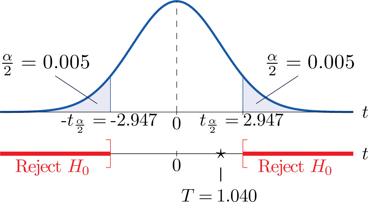
Step 4. Since the symbol in Ha is “≠” this is a two-tailed test, so there are two critical values, From the row in Figure 12.3 "Critical Values of " with the heading we read off The rejection region is
Figure 9.4 Rejection Region and Test Statistic for Note 9.13 "Example 5"
-
Step 5. As shown in Figure 9.4 "Rejection Region and Test Statistic for " the test statistic does not fall in the rejection region. The decision is not to reject H0. In the context of the problem our conclusion is:
The data do not provide sufficient evidence, at the 1% level of significance, to conclude that the mean sales per month of the two designs are different.
Example 6
Perform the test of Note 9.13 "Example 5" using the p-value approach.
Solution:
The first three steps are identical to those in Note 9.13 "Example 5".
-
Step 4. Because the test is two-tailed the observed significance or p-value of the test is the double of the area of the right tail of Student’s t-distribution, with 15 degrees of freedom, that is cut off by the test statistic T = 1.040. We can only approximate this number. Looking in the row of Figure 12.3 "Critical Values of " headed , the number 1.040 is between the numbers 0.866 and 1.341, corresponding to t0.200 and t0.100.
The area cut off by t = 0.866 is 0.200 and the area cut off by t = 1.341 is 0.100. Since 1.040 is between 0.866 and 1.341 the area it cuts off is between 0.200 and 0.100. Thus the p-value (since the area must be doubled) is between 0.400 and 0.200.
-
Step 5. Since , , so the decision is not to reject the null hypothesis:
The data do not provide sufficient evidence, at the 1% level of significance, to conclude that the mean sales per month of the two designs are different.
Key Takeaways
- In the context of estimating or testing hypotheses concerning two population means, “small” samples means that at least one sample is small. In particular, even if one sample is of size 30 or more, if the other is of size less than 30 the formulas of this section must be used.
- A confidence interval for the difference in two population means is computed using a formula in the same fashion as was done for a single population mean.
Exercises
-
Construct the confidence interval for for the level of confidence and the data from independent samples given.
-
95% confidence,
, ,
, ,
-
99% confidence,
, ,
, ,
-
-
Construct the confidence interval for for the level of confidence and the data from independent samples given.
-
90% confidence,
, ,
, ,
-
99% confidence,
, ,
, ,
-
-
Construct the confidence interval for for the level of confidence and the data from independent samples given.
-
99.9% confidence,
, ,
, ,
-
99% confidence,
, ,
, ,
-
-
Construct the confidence interval for for the level of confidence and the data from independent samples given.
-
99.5% confidence,
, ,
, ,
-
99.9% confidence,
, ,
, ,
-
-
Perform the test of hypotheses indicated, using the data from independent samples given. Use the critical value approach.
-
Test vs. @ ,
, ,
, ,
-
Test vs. @ ,
, ,
, ,
-
-
Perform the test of hypotheses indicated, using the data from independent samples given. Use the critical value approach.
-
Test vs. @ ,
, ,
, ,
-
Test vs. @ ,
, ,
, ,
-
-
Perform the test of hypotheses indicated, using the data from independent samples given. Use the critical value approach.
-
Test vs. @ ,
, ,
, ,
-
Test vs. @ ,
, ,
, ,
-
-
Perform the test of hypotheses indicated, using the data from independent samples given. Use the critical value approach.
-
Test vs. @ ,
, ,
, ,
-
Test vs. @ ,
, ,
, ,
-
-
Perform the test of hypotheses indicated, using the data from independent samples given. Use the p-value approach. (The p-value can be only approximated.)
-
Test vs. @ ,
, ,
, ,
-
Test vs. @ ,
, ,
, ,
-
-
Perform the test of hypotheses indicated, using the data from independent samples given. Use the p-value approach. (The p-value can be only approximated.)
-
Test vs. @ ,
, ,
, ,
-
Test vs. @ ,
, ,
, ,
-
-
Perform the test of hypotheses indicated, using the data from independent samples given. Use the p-value approach. (The p-value can be only approximated.)
-
Test vs. @ ,
, ,
, ,
-
Test vs. @ ,
, ,
, ,
-
-
Perform the test of hypotheses indicated, using the data from independent samples given. Use the p-value approach. (The p-value can be only approximated.)
-
Test vs. @ ,
, ,
, ,
-
Test vs. @ ,
, ,
, ,
-
Basic
In all exercises for this section assume that the populations are normal and have equal standard deviations.
-
A county environmental agency suspects that the fish in a particular polluted lake have elevated mercury level. To confirm that suspicion, five striped bass in that lake were caught and their tissues were tested for mercury. For the purpose of comparison, four striped bass in an unpolluted lake were also caught and tested. The fish tissue mercury levels in mg/kg are given below.
- Construct the 95% confidence interval for the difference in the population means based on these data.
- Test, at the 5% level of significance, whether the data provide sufficient evidence to conclude that fish in the polluted lake have elevated levels of mercury in their tissue.
-
A genetic engineering company claims that it has developed a genetically modified tomato plant that yields on average more tomatoes than other varieties. A farmer wants to test the claim on a small scale before committing to a full-scale planting. Ten genetically modified tomato plants are grown from seeds along with ten other tomato plants. At the season’s end, the resulting yields in pound are recorded as below.
- Construct the 99% confidence interval for the difference in the population means based on these data.
- Test, at the 1% level of significance, whether the data provide sufficient evidence to conclude that the mean yield of the genetically modified variety is greater than that for the standard variety.
-
The coaching staff of a professional football team believes that the rushing offense has become increasingly potent in recent years. To investigate this belief, 20 randomly selected games from one year’s schedule were compared to 11 randomly selected games from the schedule five years later. The sample information on rushing yards per game (rypg) is summarized below.
n s rypg previously 20 112 24 rypg recently 11 114 21 - Construct the 95% confidence interval for the difference in the population means based on these data.
- Test, at the 5% level of significance, whether the data on rushing yards per game provide sufficient evidence to conclude that the rushing offense has become more potent in recent years.
-
The coaching staff of professional football team believes that the rushing offense has become increasingly potent in recent years. To investigate this belief, 20 randomly selected games from one year’s schedule were compared to 11 randomly selected games from the schedule five years later. The sample information on passing yards per game (pypg) is summarized below.
n s pypg previously 20 203 38 pypg recently 11 232 33 - Construct the 95% confidence interval for the difference in the population means based on these data.
- Test, at the 5% level of significance, whether the data on passing yards per game provide sufficient evidence to conclude that the passing offense has become more potent in recent years.
-
A university administrator wishes to know if there is a difference in average starting salary for graduates with master’s degrees in engineering and those with master’s degrees in business. Fifteen recent graduates with master’s degree in engineering and 11 with master’s degrees in business are surveyed and the results are summarized below.
n s Engineering 15 68,535 1627 Business 11 63,230 2033 - Construct the 90% confidence interval for the difference in the population means based on these data.
- Test, at the 10% level of significance, whether the data provide sufficient evidence to conclude that the average starting salaries are different.
-
A gardener sets up a flower stand in a busy business district and sells bouquets of assorted fresh flowers on weekdays. To find a more profitable pricing, she sells bouquets for 15 dollars each for ten days, then for 10 dollars each for five days. Her average daily profit for the two different prices are given below.
n s $15 10 171 26 $10 5 198 29 - Construct the 90% confidence interval for the difference in the population means based on these data.
- Test, at the 10% level of significance, whether the data provide sufficient evidence to conclude the gardener’s average daily profit will be higher if the bouquets are sold at $10 each.
Applications
Answers
-
- ,
-
-
- ,
-
-
- T = 2.787, , reject H0,
- T = 1.831, , do not reject H0
-
-
- , , reject H0,
- T = 1.411, , do not reject H0
-
-
- T = 2.411, , , do not reject H0,
- T = 1.473, , , reject H0
-
-
- T = 2.827, , , reject H0.
- T = 1.699, , , reject H0
-
-
- ,
- T = 3.635, , , reject H0 (elevated levels)
-
-
- ,
- , , , do not reject H0 (not more potent)
-
-
- ,
- T = 7.395, , , reject H0 (different)
-
9.3 Comparison of Two Population Means: Paired Samples
Learning Objectives
- To learn the distinction between independent samples and paired samples.
- To learn how to construct a confidence interval for the difference in the means of two distinct populations using paired samples.
- To learn how to perform a test of hypotheses concerning the difference in the means of two distinct populations using paired samples.
Suppose chemical engineers wish to compare the fuel economy obtained by two different formulations of gasoline. Since fuel economy varies widely from car to car, if the mean fuel economy of two independent samples of vehicles run on the two types of fuel were compared, even if one formulation were better than the other the large variability from vehicle to vehicle might make any difference arising from difference in fuel difficult to detect. Just imagine one random sample having many more large vehicles than the other. Instead of independent random samples, it would make more sense to select pairs of cars of the same make and model and driven under similar circumstances, and compare the fuel economy of the two cars in each pair. Thus the data would look something like Table 9.1 "Fuel Economy of Pairs of Vehicles", where the first car in each pair is operated on one formulation of the fuel (call it Type 1 gasoline) and the second car is operated on the second (call it Type 2 gasoline).
Table 9.1 Fuel Economy of Pairs of Vehicles
| Make and Model | Car 1 | Car 2 |
|---|---|---|
| Buick LaCrosse | 17.0 | 17.0 |
| Dodge Viper | 13.2 | 12.9 |
| Honda CR-Z | 35.3 | 35.4 |
| Hummer H 3 | 13.6 | 13.2 |
| Lexus RX | 32.7 | 32.5 |
| Mazda CX-9 | 18.4 | 18.1 |
| Saab 9-3 | 22.5 | 22.5 |
| Toyota Corolla | 26.8 | 26.7 |
| Volvo XC 90 | 15.1 | 15.0 |
The first column of numbers form a sample from Population 1, the population of all cars operated on Type 1 gasoline; the second column of numbers form a sample from Population 2, the population of all cars operated on Type 2 gasoline. It would be incorrect to analyze the data using the formulas from the previous section, however, since the samples were not drawn independently. What is correct is to compute the difference in the numbers in each pair (subtracting in the same order each time) to obtain the third column of numbers as shown in Table 9.2 "Fuel Economy of Pairs of Vehicles" and treat the differences as the data. At this point, the new sample of differences in the third column of Table 9.2 "Fuel Economy of Pairs of Vehicles" may be considered as a random sample of size n = 9 selected from a population with mean This approach essentially transforms the paired two-sample problem into a one-sample problem as discussed in the previous two chapters.
Table 9.2 Fuel Economy of Pairs of Vehicles
| Make and Model | Car 1 | Car 2 | Difference |
|---|---|---|---|
| Buick LaCrosse | 17.0 | 17.0 | 0.0 |
| Dodge Viper | 13.2 | 12.9 | 0.3 |
| Honda CR-Z | 35.3 | 35.4 | −0.1 |
| Hummer H 3 | 13.6 | 13.2 | 0.4 |
| Lexus RX | 32.7 | 32.5 | 0.2 |
| Mazda CX-9 | 18.4 | 18.1 | 0.3 |
| Saab 9-3 | 22.5 | 22.5 | 0.0 |
| Toyota Corolla | 26.8 | 26.7 | 0.1 |
| Volvo XC 90 | 15.1 | 15.0 | 0.1 |
Note carefully that although it does not matter what order the subtraction is done, it must be done in the same order for all pairs. This is why there are both positive and negative quantities in the third column of numbers in Table 9.2 "Fuel Economy of Pairs of Vehicles".
Confidence Intervals
When the population of differences is normally distributed the following formula for a confidence interval for is valid.
Confidence Interval for the Difference Between Two Population Means: Paired Difference Samples
where there are n pairs, is the mean and sd is the standard deviation of their differences.
The number of degrees of freedom is
The population of differences must be normally distributed.
Example 7
Using the data in Table 9.1 "Fuel Economy of Pairs of Vehicles" construct a point estimate and a 95% confidence interval for the difference in average fuel economy between cars operated on Type 1 gasoline and cars operated on Type 2 gasoline.
Solution:
We have referred to the data in Table 9.1 "Fuel Economy of Pairs of Vehicles" because that is the way that the data are typically presented, but we emphasize that with paired sampling one immediately computes the differences, as given in Table 9.2 "Fuel Economy of Pairs of Vehicles", and uses the differences as the data.
The mean and standard deviation of the differences are
The point estimate of is
In words, we estimate that the average fuel economy of cars using Type 1 gasoline is 0.14 mpg greater than the average fuel economy of cars using Type 2 gasoline.
To apply the formula for the confidence interval, we must find The 95% confidence level means that so that From Figure 12.3 "Critical Values of ", in the row with the heading we read that Thus
We are 95% confident that the difference in the population means lies in the interval , in the sense that in repeated sampling 95% of all intervals constructed from the sample data in this manner will contain Stated differently, we are 95% confident that mean fuel economy is between 0.01 and 0.27 mpg greater with Type 1 gasoline than with Type 2 gasoline.
Hypothesis Testing
Testing hypotheses concerning the difference of two population means using paired difference samples is done precisely as it is done for independent samples, although now the null and alternative hypotheses are expressed in terms of instead of Thus the null hypothesis will always be written
The three forms of the alternative hypothesis, with the terminology for each case, are:
| Form of | Terminology |
|---|---|
| Left-tailed | |
| Right-tailed | |
| Two-tailed |
The same conditions on the population of differences that was required for constructing a confidence interval for the difference of the means must also be met when hypotheses are tested. Here is the standardized test statistic that is used in the test.
Standardized Test Statistic for Hypothesis Tests Concerning the Difference Between Two Population Means: Paired Difference Samples
where there are n pairs, is the mean and sd is the standard deviation of their differences.
The test statistic has Student’s t-distribution with degrees of freedom.
The population of differences must be normally distributed.
Example 8
Using the data of Table 9.2 "Fuel Economy of Pairs of Vehicles" test the hypothesis that mean fuel economy for Type 1 gasoline is greater than that for Type 2 gasoline against the null hypothesis that the two formulations of gasoline yield the same mean fuel economy. Test at the 5% level of significance using the critical value approach.
Solution:
The only part of the table that we use is the third column, the differences.
-
Step 1. Since the differences were computed in the order , better fuel economy with Type 1 fuel corresponds to Thus the test is
(If the differences had been computed in the opposite order then the alternative hypotheses would have been )
-
Step 2. Since the sampling is in pairs the test statistic is
-
Step 3. We have already computed and sd in the previous example. Inserting their values and into the formula for the test statistic gives
- Step 4. Since the symbol in Ha is “>” this is a right-tailed test, so there is a single critical value, with 8 degrees of freedom, which from the row labeled in Figure 12.3 "Critical Values of " we read off as 1.860. The rejection region is
-
Step 5. As shown in Figure 9.5 "Rejection Region and Test Statistic for " the test statistic falls in the rejection region. The decision is to reject H0. In the context of the problem our conclusion is:
Figure 9.5 Rejection Region and Test Statistic for Note 9.20 "Example 8"
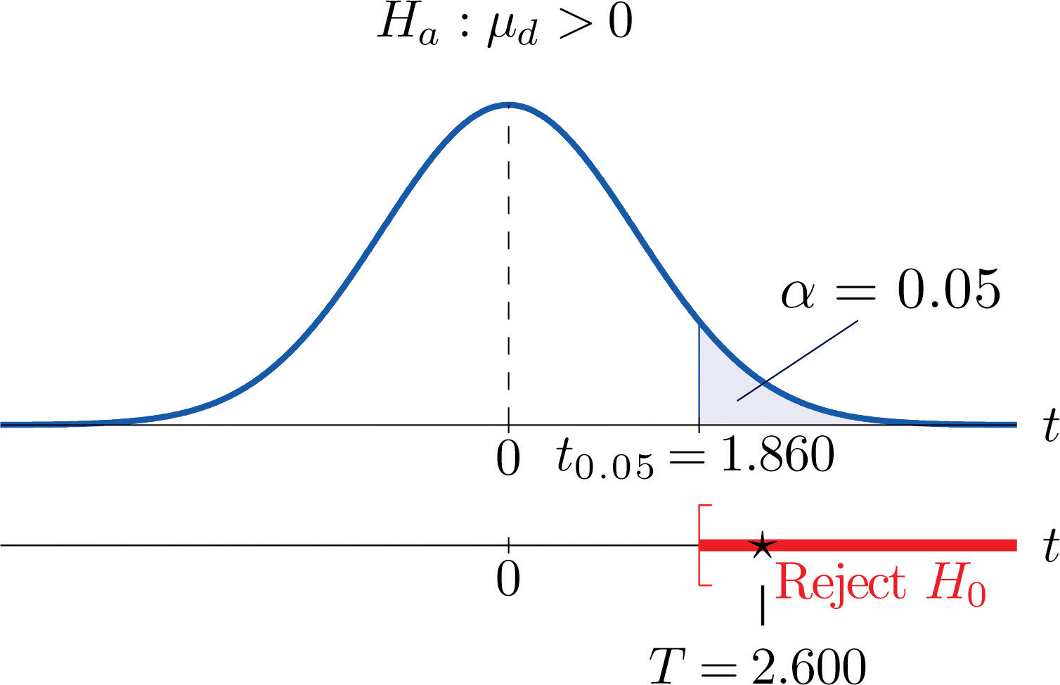
The data provide sufficient evidence, at the 5% level of significance, to conclude that the mean fuel economy provided by Type 1 gasoline is greater than that for Type 2 gasoline.
Example 9
Perform the test of Note 9.20 "Example 8" using the p-value approach.
Solution:
The first three steps are identical to those in Note 9.20 "Example 8".
-
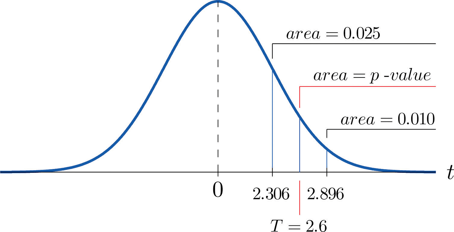
Step 4. Because the test is one-tailed the observed significance or p-value of the test is just the area of the right tail of Student’s t-distribution, with 8 degrees of freedom, that is cut off by the test statistic T = 2.600. We can only approximate this number. Looking in the row of Figure 12.3 "Critical Values of " headed , the number 2.600 is between the numbers 2.306 and 2.896, corresponding to t0.025 and t0.010.
The area cut off by t = 2.306 is 0.025 and the area cut off by t = 2.896 is 0.010. Since 2.600 is between 2.306 and 2.896 the area it cuts off is between 0.025 and 0.010. Thus the p-value is between 0.025 and 0.010. In particular it is less than 0.025. See Figure 9.6.
Figure 9.6 P-Value for Note 9.21 "Example 9"
-
Step 5. Since 0.025 < 0.05, so the decision is to reject the null hypothesis:
The data provide sufficient evidence, at the 5% level of significance, to conclude that the mean fuel economy provided by Type 1 gasoline is greater than that for Type 2 gasoline.
The paired two-sample experiment is a very powerful study design. It bypasses many unwanted sources of “statistical noise” that might otherwise influence the outcome of the experiment, and focuses on the possible difference that might arise from the one factor of interest.
If the sample is large (meaning that n ≥ 30) then in the formula for the confidence interval we may replace by For hypothesis testing when the number of pairs is at least 30, we may use the same statistic as for small samples for hypothesis testing, except now it follows a standard normal distribution, so we use the last line of Figure 12.3 "Critical Values of " to compute critical values, and p-values can be computed exactly with Figure 12.2 "Cumulative Normal Probability", not merely estimated using Figure 12.3 "Critical Values of ".
Key Takeaways
- When the data are collected in pairs, the differences computed for each pair are the data that are used in the formulas.
- A confidence interval for the difference in two population means using paired sampling is computed using a formula in the same fashion as was done for a single population mean.
- The same five-step procedure used to test hypotheses concerning a single population mean is used to test hypotheses concerning the difference between two population means using pair sampling. The only difference is in the formula for the standardized test statistic.
Exercises
-
Use the following paired sample data for this exercise.
- Compute and sd.
- Give a point estimate for
- Construct the 95% confidence interval for from these data.
- Test, at the 10% level of significance, the hypothesis that as an alternative to the null hypothesis that
-
Use the following paired sample data for this exercise.
- Compute and sd.
- Give a point estimate for
- Construct the 90% confidence interval for from these data.
- Test, at the 1% level of significance, the hypothesis that as an alternative to the null hypothesis that
-
Use the following paired sample data for this exercise.
- Compute and sd.
- Give a point estimate for
- Construct the 99% confidence interval for from these data.
- Test, at the 10% level of significance, the hypothesis that as an alternative to the null hypothesis that
-
Use the following paired sample data for this exercise.
- Compute and sd.
- Give a point estimate for
- Construct the 98% confidence interval for from these data.
- Test, at the 2% level of significance, the hypothesis that as an alternative to the null hypothesis that
Basic
In all exercises for this section assume that the population of differences is normal.
-
Each of five laboratory mice was released into a maze twice. The five pairs of times to escape were:
Mouse 1 2 3 4 5 First release 129 89 136 163 118 Second release 113 97 139 85 75 - Compute and sd.
- Give a point estimate for
- Construct the 90% confidence interval for from these data.
- Test, at the 10% level of significance, the hypothesis that it takes mice less time to run the maze on the second trial, on average.
-
Eight golfers were asked to submit their latest scores on their favorite golf courses. These golfers were each given a set of newly designed clubs. After playing with the new clubs for a few months, the golfers were again asked to submit their latest scores on the same golf courses. The results are summarized below.
Golfer 1 2 3 4 5 6 7 8 Own clubs 77 80 69 73 73 72 75 77 New clubs 72 81 68 73 75 70 73 75 - Compute and sd.
- Give a point estimate for
- Construct the 99% confidence interval for from these data.
- Test, at the 1% level of significance, the hypothesis that on average golf scores are lower with the new clubs.
-
A neighborhood home owners association suspects that the recent appraisal values of the houses in the neighborhood conducted by the county government for taxation purposes is too high. It hired a private company to appraise the values of ten houses in the neighborhood. The results, in thousands of dollars, are
House County Government Private Company 1 217 219 2 350 338 3 296 291 4 237 237 5 237 235 6 272 269 7 257 239 8 277 275 9 312 320 10 335 335 - Give a point estimate for the difference between the mean private appraisal of all such homes and the government appraisal of all such homes.
- Construct the 99% confidence interval based on these data for the difference.
- Test, at the 1% level of significance, the hypothesis that appraised values by the county government of all such houses is greater than the appraised values by the private appraisal company.
-
In order to cut costs a wine producer is considering using duo or 1 + 1 corks in place of full natural wood corks, but is concerned that it could affect buyers’s perception of the quality of the wine. The wine producer shipped eight pairs of bottles of its best young wines to eight wine experts. Each pair includes one bottle with a natural wood cork and one with a duo cork. The experts are asked to rate the wines on a one to ten scale, higher numbers corresponding to higher quality. The results are:
Wine Expert Duo Cork Wood Cork 1 8.5 8.5 2 8.0 8.5 3 6.5 8.0 4 7.5 8.5 5 8.0 7.5 6 8.0 8.0 7 9.0 9.0 8 7.0 7.5 - Give a point estimate for the difference between the mean ratings of the wine when bottled are sealed with different kinds of corks.
- Construct the 90% confidence interval based on these data for the difference.
- Test, at the 10% level of significance, the hypothesis that on the average duo corks decrease the rating of the wine.
-
Engineers at a tire manufacturing corporation wish to test a new tire material for increased durability. To test the tires under realistic road conditions, new front tires are mounted on each of 11 company cars, one tire made with a production material and the other with the experimental material. After a fixed period the 11 pairs were measured for wear. The amount of wear for each tire (in mm) is shown in the table:
Car Production Experimental 1 5.1 5.0 2 6.5 6.5 3 3.6 3.1 4 3.5 3.7 5 5.7 4.5 6 5.0 4.1 7 6.4 5.3 8 4.7 2.6 9 3.2 3.0 10 3.5 3.5 11 6.4 5.1 - Give a point estimate for the difference in mean wear.
- Construct the 99% confidence interval for the difference based on these data.
- Test, at the 1% level of significance, the hypothesis that the mean wear with the experimental material is less than that for the production material.
-
A marriage counselor administered a test designed to measure overall contentment to 30 randomly selected married couples. The scores for each couple are given below. A higher number corresponds to greater contentment or happiness.
Couple Husband Wife 1 47 44 2 44 46 3 49 44 4 53 44 5 42 43 6 45 45 7 48 47 8 45 44 9 52 44 10 47 42 11 40 34 12 45 42 13 40 43 14 46 41 15 47 45 16 46 45 17 46 41 18 46 41 19 44 45 20 45 43 21 48 38 22 42 46 23 50 44 24 46 51 25 43 45 26 50 40 27 46 46 28 42 41 29 51 41 30 46 47 - Test, at the 1% level of significance, the hypothesis that on average men and women are not equally happy in marriage.
- Test, at the 1% level of significance, the hypothesis that on average men are happier than women in marriage.
Applications
-
Large Data Set 5 lists the scores for 25 randomly selected students on practice SAT reading tests before and after taking a two-week SAT preparation course. Denote the population of all students who have taken the course as Population 1 and the population of all students who have not taken the course as Population 2.
http://www.flatworldknowledge.com/sites/all/files/data5.xls
- Compute the 25 differences in the order , their mean , and their sample standard deviation sd.
- Give a point estimate for , the difference in the mean score of all students who have taken the course and the mean score of all who have not.
- Construct a 98% confidence interval for
- Test, at the 1% level of significance, the hypothesis that the mean SAT score increases by at least ten points by taking the two-week preparation course.
-
Large Data Set 12 lists the scores on one round for 75 randomly selected members at a golf course, first using their own original clubs, then two months later after using new clubs with an experimental design. Denote the population of all golfers using their own original clubs as Population 1 and the population of all golfers using the new style clubs as Population 2.
http://www.flatworldknowledge.com/sites/all/files/data12.xls
- Compute the 75 differences in the order , their mean , and their sample standard deviation sd.
- Give a point estimate for , the difference in the mean score of all golfers using their original clubs and the mean score of all golfers using the new kind of clubs.
- Construct a 90% confidence interval for
- Test, at the 1% level of significance, the hypothesis that the mean golf score decreases by at least one stroke by using the new kind of clubs.
-
Consider the previous problem again. Since the data set is so large, it is reasonable to use the standard normal distribution instead of Student’s t-distribution with 74 degrees of freedom.
- Construct a 90% confidence interval for using the standard normal distribution, meaning that the formula is (The computations done in part (a) of the previous problem still apply and need not be redone.) How does the result obtained here compare to the result obtained in part (c) of the previous problem?
- Test, at the 1% level of significance, the hypothesis that the mean golf score decreases by at least one stroke by using the new kind of clubs, using the standard normal distribution. (All the work done in part (d) of the previous problem applies, except the critical value is now instead of (or the p-value can be computed exactly instead of only approximated, if you used the p-value approach).) How does the result obtained here compare to the result obtained in part (c) of the previous problem?
- Construct the 99% confidence intervals for using both the and distributions. How much difference is there in the results now?
Large Data Set Exercises
Answers
-
- , ,
- ,
- ,
- T = 1.162, , , do not reject H0
-
-
- , ,
- ,
- ,
- , , , reject H0
-
-
- , ,
- 25.2,
- T = 1.580, , , reject H0 (takes less time)
-
-
- 3.2,
- T = 1.392, , , do not reject H0 (government appraisals not higher)
-
-
- 0.65,
- ,
- T = 3.014, , , reject H0 (experimental material wears less)
-
-
- and
- vs. Test Statistic: T = 3.1014. Rejection Region: Decision: Reject H0.
-
-
- Endpoints change in the third deciaml place.
- vs. Test Statistic: Z = 3.6791. Rejection Region: Decision: Reject H0. The decision is the same as in the previous problem.
- Using the distribution, Using the distribution, There is a difference.
9.4 Comparison of Two Population Proportions
Learning Objectives
- To learn how to construct a confidence interval for the difference in the proportions of two distinct populations that have a particular characteristic of interest.
- To learn how to perform a test of hypotheses concerning the difference in the proportions of two distinct populations that have a particular characteristic of interest.
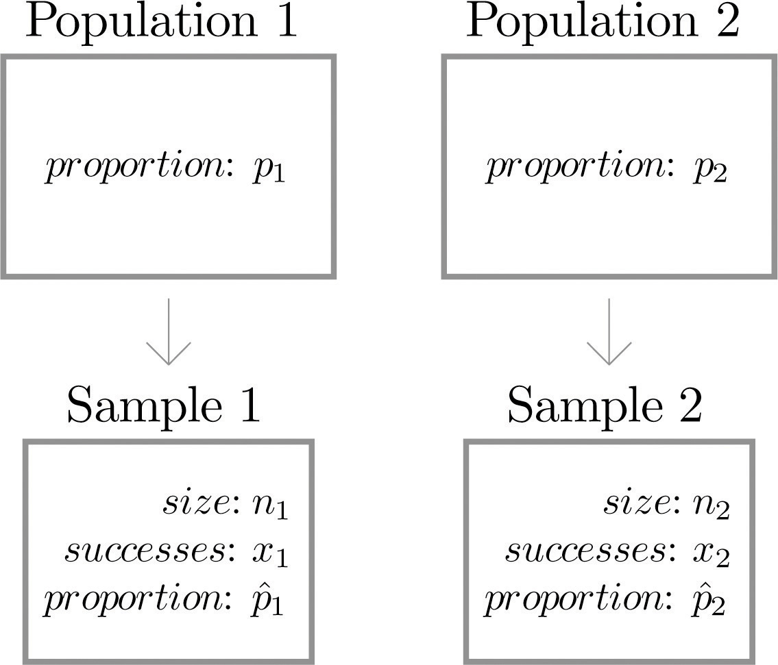
Suppose we wish to compare the proportions of two populations that have a specific characteristic, such as the proportion of men who are left-handed compared to the proportion of women who are left-handed. Figure 9.7 "Independent Sampling from Two Populations In Order to Compare Proportions" illustrates the conceptual framework of our investigation. Each population is divided into two groups, the group of elements that have the characteristic of interest (for example, being left-handed) and the group of elements that do not. We arbitrarily label one population as Population 1 and the other as Population 2, and subscript the proportion of each population that possesses the characteristic with the number 1 or 2 to tell them apart. We draw a random sample from Population 1 and label the sample statistic it yields with the subscript 1. Without reference to the first sample we draw a sample from Population 2 and label its sample statistic with the subscript 2.
Figure 9.7 Independent Sampling from Two Populations In Order to Compare Proportions
Our goal is to use the information in the samples to estimate the difference in the two population proportions and to make statistically valid inferences about it.
Confidence Intervals
Since the sample proportion computed using the sample drawn from Population 1 is a good estimator of population proportion p1 of Population 1 and the sample proportion computed using the sample drawn from Population 2 is a good estimator of population proportion p2 of Population 2, a reasonable point estimate of the difference is In order to widen this point estimate into a confidence interval we suppose that both samples are large, as described in Section 7.3 "Large Sample Estimation of a Population Proportion" in Chapter 7 "Estimation" and repeated below. If so, then the following formula for a confidence interval for is valid.
Confidence Interval for the Difference Between Two Population Proportions
The samples must be independent, and each sample must be large: each of the intervals
and
must lie wholly within the interval
Example 10
The department of code enforcement of a county government issues permits to general contractors to work on residential projects. For each permit issued, the department inspects the result of the project and gives a “pass” or “fail” rating. A failed project must be re-inspected until it receives a pass rating. The department had been frustrated by the high cost of re-inspection and decided to publish the inspection records of all contractors on the web. It was hoped that public access to the records would lower the re-inspection rate. A year after the web access was made public, two samples of records were randomly selected. One sample was selected from the pool of records before the web publication and one after. The proportion of projects that passed on the first inspection was noted for each sample. The results are summarized below. Construct a point estimate and a 90% confidence interval for the difference in the passing rate on first inspection between the two time periods.
Solution:
The point estimate of is
Because the “No public web access” population was labeled as Population 1 and the “Public web access” population was labeled as Population 2, in words this means that we estimate that the proportion of projects that passed on the first inspection increased by 13 percentage points after records were posted on the web.
The sample sizes are sufficiently large for constructing a confidence interval since for sample 1:
so that
and for sample 2:
so that
To apply the formula for the confidence interval, we first observe that the 90% confidence level means that so that From Figure 12.3 "Critical Values of " we read directly that Thus the desired confidence interval is
The 90% confidence interval is We are 90% confident that the difference in the population proportions lies in the interval , in the sense that in repeated sampling 90% of all intervals constructed from the sample data in this manner will contain Taking into account the labeling of the two populations, this means that we are 90% confident that the proportion of projects that pass on the first inspection is between 6 and 20 percentage points higher after public access to the records than before.
Hypothesis Testing
In hypothesis tests concerning the relative sizes of the proportions p1 and p2 of two populations that possess a particular characteristic, the null and alternative hypotheses will always be expressed in terms of the difference of the two population proportions. Hence the null hypothesis is always written
The three forms of the alternative hypothesis, with the terminology for each case, are:
| Form of | Terminology |
|---|---|
| Left-tailed | |
| Right-tailed | |
| Two-tailed |
As long as the samples are independent and both are large the following formula for the standardized test statistic is valid, and it has the standard normal distribution.
Standardized Test Statistic for Hypothesis Tests Concerning the Difference Between Two Population Proportions
The test statistic has the standard normal distribution.
The samples must be independent, and each sample must be large: each of the intervals
and
must lie wholly within the interval
Example 11
Using the data of Note 9.25 "Example 10", test whether there is sufficient evidence to conclude that public web access to the inspection records has increased the proportion of projects that passed on the first inspection by more than 5 percentage points. Use the critical value approach at the 10% level of significance.
Solution:
-
Step 1. Taking into account the labeling of the populations an increase in passing rate at the first inspection by more than 5 percentage points after public access on the web may be expressed as , which by algebra is the same as This is the alternative hypothesis. Since the null hypothesis is always expressed as an equality, with the same number on the right as is in the alternative hypothesis, the test is
-
Step 2. Since the test is with respect to a difference in population proportions the test statistic is
-
Step 3. Inserting the values given in Note 9.25 "Example 10" and the value into the formula for the test statistic gives
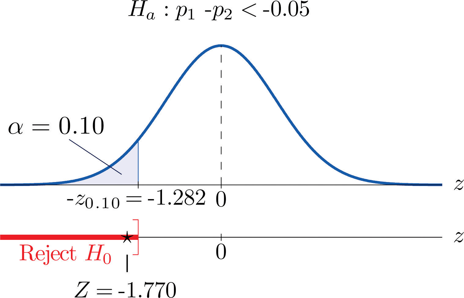
- Step 4. Since the symbol in Ha is “<” this is a left-tailed test, so there is a single critical value, From the last row in Figure 12.3 "Critical Values of " , so The rejection region is
-
Step 5. As shown in Figure 9.8 "Rejection Region and Test Statistic for " the test statistic falls in the rejection region. The decision is to reject H0. In the context of the problem our conclusion is:
The data provide sufficient evidence, at the 10% level of significance, to conclude that the rate of passing on the first inspection has increased by more than 5 percentage points since records were publicly posted on the web.
Figure 9.8 Rejection Region and Test Statistic for Note 9.27 "Example 11"
Example 12
Perform the test of Note 9.27 "Example 11" using the p-value approach.
Solution:
The first three steps are identical to those in Note 9.27 "Example 11".
- Step 4. Because the test is left-tailed the observed significance or p-value of the test is just the area of the left tail of the standard normal distribution that is cut off by the test statistic From Figure 12.2 "Cumulative Normal Probability" the area of the left tail determined by −1.77 is 0.0384. The p-value is 0.0384.
- Step 5. Since the p-value 0.0384 is less than , the decision is to reject the null hypothesis: The data provide sufficient evidence, at the 10% level of significance, to conclude that the rate of passing on the first inspection has increased by more than 5 percentage points since records were publicly posted on the web.
Finally a common misuse of the formulas given in this section must be mentioned. Suppose a large pre-election survey of potential voters is conducted. Each person surveyed is asked to express a preference between, say, Candidate A and Candidate B. (Perhaps “no preference” or “other” are also choices, but that is not important.) In such a survey, estimators and of pA and pB can be calculated. It is important to realize, however, that these two estimators were not calculated from two independent samples. While may be a reasonable estimator of , the formulas for confidence intervals and for the standardized test statistic given in this section are not valid for data obtained in this manner.
Key Takeaways
- A confidence interval for the difference in two population proportions is computed using a formula in the same fashion as was done for a single population mean.
- The same five-step procedure used to test hypotheses concerning a single population proportion is used to test hypotheses concerning the difference between two population proportions. The only difference is in the formula for the standardized test statistic.
Exercises
-
Construct the confidence interval for for the level of confidence and the data given. (The samples are sufficiently large.)
-
90% confidence,
,
,
-
95% confidence,
,
,
-
-
Construct the confidence interval for for the level of confidence and the data given. (The samples are sufficiently large.)
-
98% confidence,
,
,
-
99.5% confidence,
,
,
-
-
Construct the confidence interval for for the level of confidence and the data given. (The samples are sufficiently large.)
-
80% confidence,
,
,
-
95% confidence,
,
,
-
-
Construct the confidence interval for for the level of confidence and the data given. (The samples are sufficiently large.)
-
99% confidence,
,
,
-
95% confidence,
,
,
-
-
Perform the test of hypotheses indicated, using the data given. Use the critical value approach. Compute the p-value of the test as well. (The samples are sufficiently large.)
-
Test vs. @ ,
,
,
-
Test vs. @ ,
,
,
-
-
Perform the test of hypotheses indicated, using the data given. Use the critical value approach. Compute the p-value of the test as well. (The samples are sufficiently large.)
-
Test vs. @ ,
,
,
-
Test vs. @ ,
,
,
-
-
Perform the test of hypotheses indicated, using the data given. Use the critical value approach. Compute the p-value of the test as well. (The samples are sufficiently large.)
-
Test vs. @ ,
,
,
-
Test vs. @ ,
,
,
-
-
Perform the test of hypotheses indicated, using the data given. Use the critical value approach. Compute the p-value of the test as well. (The samples are sufficiently large.)
-
Test vs. @ ,
,
,
-
Test vs. @ ,
,
,
-
-
Perform the test of hypotheses indicated, using the data given. Use the p-value approach. (The samples are sufficiently large.)
-
Test vs. @ ,
,
,
-
Test vs. @ ,
,
,
-
-
Perform the test of hypotheses indicated, using the data given. Use the p-value approach. (The samples are sufficiently large.)
-
Test vs. @ ,
,
,
-
Test vs. @ ,
,
,
-
-
Perform the test of hypotheses indicated, using the data given. Use the p-value approach. (The samples are sufficiently large.)
-
Test vs. @ ,
,
,
-
Test vs. @ ,
,
,
-
-
Perform the test of hypotheses indicated, using the data given. Use the p-value approach. (The samples are sufficiently large.)
-
Test vs. @ ,
,
,
-
Test vs. @ ,
,
,
-
Basic
-
Voters in a particular city who identify themselves with one or the other of two political parties were randomly selected and asked if they favor a proposal to allow citizens with proper license to carry a concealed handgun in city parks. The results are:
Party A Party B Sample size, n 150 200 Number in favor, x 90 140 - Give a point estimate for the difference in the proportion of all members of Party A and all members of Party B who favor the proposal.
- Construct the 95% confidence interval for the difference, based on these data.
- Test, at the 5% level of significance, the hypothesis that the proportion of all members of Party A who favor the proposal is less than the proportion of all members of Party B who do.
- Compute the p-value of the test.
-
To investigate a possible relation between gender and handedness, a random sample of 320 adults was taken, with the following results:
Men Women Sample size, n 168 152 Number of left-handed, x 24 9 - Give a point estimate for the difference in the proportion of all men who are left-handed and the proportion of all women who are left-handed.
- Construct the 95% confidence interval for the difference, based on these data.
- Test, at the 5% level of significance, the hypothesis that the proportion of men who are left-handed is greater than the proportion of women who are.
- Compute the p-value of the test.
-
A local school board member randomly sampled private and public high school teachers in his district to compare the proportions of National Board Certified (NBC) teachers in the faculty. The results were:
Private Schools Public Schools Sample size, n 80 520 Proportion of NBC teachers, 0.175 0.150 - Give a point estimate for the difference in the proportion of all teachers in area public schools and the proportion of all teachers in private schools who are National Board Certified.
- Construct the 90% confidence interval for the difference, based on these data.
- Test, at the 10% level of significance, the hypothesis that the proportion of all public school teachers who are National Board Certified is less than the proportion of private school teachers who are.
- Compute the p-value of the test.
-
In professional basketball games, the fans of the home team always try to distract free throw shooters on the visiting team. To investigate whether this tactic is actually effective, the free throw statistics of a professional basketball player with a high free throw percentage were examined. During the entire last season, this player had 656 free throws, 420 in home games and 236 in away games. The results are summarized below.
Home Away Sample size, n 420 236 Free throw percent, 81.5% 78.8% - Give a point estimate for the difference in the proportion of free throws made at home and away.
- Construct the 90% confidence interval for the difference, based on these data.
- Test, at the 10% level of significance, the hypothesis that there exists a home advantage in free throws.
- Compute the p-value of the test.
-
Randomly selected middle-aged people in both China and the United States were asked if they believed that adults have an obligation to financially support their aged parents. The results are summarized below.
China USA Sample size, n 1300 150 Number of yes, x 1170 110 Test, at the 1% level of significance, whether the data provide sufficient evidence to conclude that there exists a cultural difference in attitude regarding this question.
-
A manufacturer of walk-behind push mowers receives refurbished small engines from two new suppliers, A and B. It is not uncommon that some of the refurbished engines need to be lightly serviced before they can be fitted into mowers. The mower manufacturer recently received 100 engines from each supplier. In the shipment from A, 13 needed further service. In the shipment from B, 10 needed further service. Test, at the 10% level of significance, whether the data provide sufficient evidence to conclude that there exists a difference in the proportions of engines from the two suppliers needing service.
Applications
In all the remaining exercsises the samples are sufficiently large (so this need not be checked).
-
Large Data Sets 6A and 6B record results of a random survey of 200 voters in each of two regions, in which they were asked to express whether they prefer Candidate A for a U.S. Senate seat or prefer some other candidate. Let the population of all voters in region 1 be denoted Population 1 and the population of all voters in region 2 be denoted Population 2. Let p1 be the proportion of voters in Population 1 who prefer Candidate A, and p2 the proportion in Population 2 who do.
http://www.flatworldknowledge.com/sites/all/files/data6A.xls
http://www.flatworldknowledge.com/sites/all/files/data6B.xls
- Find the relevant sample proportions and
- Construct a point estimate for
- Construct a 95% confidence interval for
- Test, at the 5% level of significance, the hypothesis that the same proportion of voters in the two regions favor Candidate A, against the alternative that a larger proportion in Population 2 do.
-
Large Data Set 11 records the results of samples of real estate sales in a certain region in the year 2008 (lines 2 through 536) and in the year 2010 (lines 537 through 1106). Foreclosure sales are identified with a 1 in the second column. Let all real estate sales in the region in 2008 be Population 1 and all real estate sales in the region in 2010 be Population 2.
http://www.flatworldknowledge.com/sites/all/files/data11.xls
- Use the sample data to construct point estimates and of the proportions p1 and p2 of all real estate sales in this region in 2008 and 2010 that were foreclosure sales. Construct a point estimate of
- Use the sample data to construct a 90% confidence for
- Test, at the 10% level of significance, the hypothesis that the proportion of real estate sales in the region in 2010 that were foreclosure sales was greater than the proportion of real estate sales in the region in 2008 that were foreclosure sales. (The default is that the proportions were the same.)
Large Data Set Exercises
Answers
-
- ,
-
-
- ,
-
-
- Z = 0.996, , , do not reject H0,
- , , , reject H0
-
-
- , , , reject H0,
- Z = 2.020, , , do not reject H0
-
-
- , , reject H0,
- , , do not reject H0
-
-
- Z = 1.36, , do not reject H0,
- Z = 2.32, , do not reject H0
-
-
- −0.10,
- ,
- , , reject H0 (fewer in Party A favor),
- p-value = 0.0262
-
-
- 0.025,
- ,
- Z = 0.552, , do not reject H0 (as many public school teachers are certified),
- p-value = 0.2912
-
-
Z = 4.498, , reject H0 (different)
-
-
- and
- vs. Test Statistic: Rejection Region: Decision: Fail to reject H0.
-
9.5 Sample Size Considerations
Learning Objective
- To learn how to apply formulas for estimating the size samples that will be needed in order to construct a confidence interval for the difference in two population means or proportions that meets given criteria.
As was pointed out at the beginning of Section 7.4 "Sample Size Considerations" in Chapter 7 "Estimation", sampling is typically done with definite objectives in mind. For example, a physician might wish to estimate the difference in the average amount of sleep gotten by patients suffering a certain condition with the average amount of sleep got by healthy adults, at 90% confidence and to within half an hour. Since sampling costs time, effort, and money, it would be useful to be able to estimate the smallest size samples that are likely to meet these criteria.
Estimating with Independent Samples
Assuming that large samples will be required, the confidence interval formula for estimating the difference between two population means using independent samples is , where
To say that we wish to estimate the mean to within a certain number of units means that we want the margin of error E to be no larger than that number. The number is determined by the desired level of confidence.
The numbers s1 and s2 are estimates of the standard deviations and of the two populations. In analogy with what we did in Section 7.4 "Sample Size Considerations" in Chapter 7 "Estimation" we will assume that we either know or can reasonably approximate and
We cannot solve for both n1 and n2, so we have to make an assumption about their relative sizes. We will specify that they be equal. With these assumptions we obtain the minimum sample sizes needed by solving the equation displayed just above for
Minimum Equal Sample Sizes for Estimating the Difference in the Means of Two Populations Using Independent Samples
The estimated minimum equal sample sizes needed to estimate the difference in two population means to within E units at % confidence is
In all the examples and exercises the population standard deviations and will be given.
Example 13
A law firm wishes to estimate the difference in the mean delivery time of documents sent between two of its offices by two different courier companies, to within half an hour and with 99.5% confidence. From their records it will randomly sample the same number n of documents as delivered by each courier company. Determine how large n must be if the estimated standard deviations of the delivery times are 0.75 hour for one company and 1.15 hours for the other.
Solution:
Confidence level 99.5% means that so From the last line of Figure 12.3 "Critical Values of " we obtain
To say that the estimate is to be “to within half an hour” means that E = 0.5. Thus
which we round up to 60, since it is impossible to take a fractional observation. The law firm must sample 60 document deliveries by each company.
Estimating with Paired Samples
As we mentioned at the end of Section 9.3 "Comparison of Two Population Means: Paired Samples", if the sample is large (meaning that n ≥ 30) then in the formula for the confidence interval we may replace by , so that the confidence interval formula becomes for
The number sd is an estimate of the standard deviations of the population of differences. We must assume that we either know or can reasonably approximate Thus, assuming that large samples will be required to meet the criteria given, we can solve the displayed equation for n to obtain an estimate of the number of pairs needed in the sample.
Minimum Sample Size for Estimating the Difference in the Means of Two Populations Using Paired Difference Samples
The estimated minimum number of pairs n needed to estimate the difference in two population means to within E units at % confidence using paired difference samples is
In all the examples and exercises the population standard deviation of the differences will be given.
Example 14
A automotive tire manufacturer wishes to compare the mean lifetime of two tread designs under actual driving conditions. They will mount one of each type of tire on n vehicles (both on the front or both on the back) and measure the difference in remaining tread after 20,000 miles of driving. If the standard deviation of the differences is assumed to be 0.025 inch, find the minimum samples size needed to estimate the difference in mean depth (at 20,000 miles use) to within 0.01 inch at 99.9% confidence.
Solution:
Confidence level 99.9% means that so From the last line of Figure 12.3 "Critical Values of " we obtain
To say that the estimate is to be “to within 0.01 inch” means that E = 0.01. Thus
which we round up to 68. The manufacturer must test 68 pairs of tires.
Estimating
The confidence interval formula for estimating the difference between two population proportions is , where
To say that we wish to estimate the mean to within a certain number of units means that we want the margin of error E to be no larger than that number. The number is determined by the desired level of confidence.
We cannot solve for both n1 and n2, so we have to make an assumption about their relative sizes. We will specify that they be equal. With these assumptions we obtain the minimum sample sizes needed by solving the displayed equation for
Minimum Equal Sample Sizes for Estimating the Difference in Two Population Proportions
The estimated minimum equal sample sizes needed to estimate the difference in two population proportions to within E percentage points at % confidence is
Here we face the same dilemma that we encountered in the case of a single population proportion: the formula for estimating how large a sample to take contains the numbers and , which we know only after we have taken the sample. There are two ways out of this dilemma. Typically the researcher will have some idea as to the values of the population proportions p1 and p2, hence of what the sample proportions and are likely to be. If so, those estimates can be used in the formula.
The second approach to resolving the dilemma is simply to replace each of and in the formula by 0.5. As in the one-population case, this is the most conservative estimate, since it gives the largest possible estimate of n. If we have an estimate of only one of p1 and p2 we can use that estimate for it, and use the conservative estimate 0.5 for the other.
Example 15
Find the minimum equal sample sizes necessary to construct a 98% confidence interval for the difference with a margin of error E = 0.05,
- assuming that no prior knowledge about p1 or p2 is available; and
- assuming that prior studies suggest that and
Solution:
Confidence level 98% means that so From the last line of Figure 12.3 "Critical Values of " we obtain
-
Since there is no prior knowledge of p1 or p2 we make the most conservative estimate that and Then
which we round up to 1,083. We must take a sample of size 1,083 from each population.
-
Since we estimate by 0.2, and since we estimate by 0.3. Thus we obtain
which we round up to 801. We must take a sample of size 801 from each population.
Key Takeaways
- If the population standard deviations and are known or can be estimated, then the minimum equal sizes of independent samples needed to obtain a confidence interval for the difference in two population means with a given maximum error of the estimate E and a given level of confidence can be estimated.
- If the standard deviation of the population of differences in pairs drawn from two populations is known or can be estimated, then the minimum number of sample pairs needed under paired difference sampling to obtain a confidence interval for the difference in two population means with a given maximum error of the estimate E and a given level of confidence can be estimated.
- The minimum equal sample sizes needed to obtain a confidence interval for the difference in two population proportions with a given maximum error of the estimate and a given level of confidence can always be estimated. If there is prior knowledge of the population proportions p1 and p2 then the estimate can be sharpened.
Exercises
-
Estimate the common sample size n of equally sized independent samples needed to estimate as specified when the population standard deviations are as shown.
- 90% confidence, to within 3 units, and
- 99% confidence, to within 4 units, and
- 95% confidence, to within 5 units, and
-
Estimate the common sample size n of equally sized independent samples needed to estimate as specified when the population standard deviations are as shown.
- 80% confidence, to within 2 units, and
- 90% confidence, to within 0.3 units, and
- 99% confidence, to within 11 units, and
-
Estimate the number n of pairs that must be sampled in order to estimate as specified when the standard deviation sd of the population of differences is as shown.
- 80% confidence, to within 6 units,
- 95% confidence, to within 4 units,
- 90% confidence, to within 5.2 units,
-
Estimate the number n of pairs that must be sampled in order to estimate as specified when the standard deviation sd of the population of differences is as shown.
- 90% confidence, to within 20 units,
- 95% confidence, to within 11 units,
- 99% confidence, to within 1.8 units,
-
Estimate the minimum equal sample sizes necessary in order to estimate as specified.
-
80% confidence, to within 0.05 (five percentage points)
- when no prior knowledge of p1 or p2 is available
- when prior studies indicate that and
-
90% confidence, to within 0.02 (two percentage points)
- when no prior knowledge of p1 or p2 is available
- when prior studies indicate that and
-
95% confidence, to within 0.10 (ten percentage points)
- when no prior knowledge of p1 or p2 is available
- when prior studies indicate that and
-
-
Estimate the minimum equal sample sizes necessary in order to estimate as specified.
-
80% confidence, to within 0.02 (two percentage points)
- when no prior knowledge of p1 or p2 is available
- when prior studies indicate that and
-
90% confidence, to within 0.05 (two percentage points)
- when no prior knowledge of p1 or p2 is available
- when prior studies indicate that and
-
95% confidence, to within 0.10 (ten percentage points)
- when no prior knowledge of p1 or p2 is available
- when prior studies indicate that and
-
Basic
-
An educational researcher wishes to estimate the difference in average scores of elementary school children on two versions of a 100-point standardized test, at 99% confidence and to within two points. Estimate the minimum equal sample sizes necessary if it is known that the standard deviation of scores on different versions of such tests is 4.9.
-
A university administrator wishes to estimate the difference in mean grade point averages among all men affiliated with fraternities and all unaffiliated men, with 95% confidence and to within 0.15. It is known from prior studies that the standard deviations of grade point averages in the two groups have common value 0.4. Estimate the minimum equal sample sizes necessary to meet these criteria.
-
An automotive tire manufacturer wishes to estimate the difference in mean wear of tires manufactured with an experimental material and ordinary production tire, with 90% confidence and to within 0.5 mm. To eliminate extraneous factors arising from different driving conditions the tires will be tested in pairs on the same vehicles. It is known from prior studies that the standard deviations of the differences of wear of tires constructed with the two kinds of materials is 1.75 mm. Estimate the minimum number of pairs in the sample necessary to meet these criteria.
-
To assess to the relative happiness of men and women in their marriages, a marriage counselor plans to administer a test measuring happiness in marriage to n randomly selected married couples, record the their test scores, find the differences, and then draw inferences on the possible difference. Let and be the true average levels of happiness in marriage for men and women respectively as measured by this test. Suppose it is desired to find a 90% confidence interval for estimating to within two test points. Suppose further that, from prior studies, it is known that the standard deviation of the differences in test scores is What is the minimum number of married couples that must be included in this study?
-
A journalist plans to interview an equal number of members of two political parties to compare the proportions in each party who favor a proposal to allow citizens with a proper license to carry a concealed handgun in public parks. Let p1 and p2 be the true proportions of members of the two parties who are in favor of the proposal. Suppose it is desired to find a 95% confidence interval for estimating to within 0.05. Estimate the minimum equal number of members of each party that must be sampled to meet these criteria.
-
A member of the state board of education wants to compare the proportions of National Board Certified (NBC) teachers in private high schools and in public high schools in the state. His study plan calls for an equal number of private school teachers and public school teachers to be included in the study. Let p1 and p2 be these proportions. Suppose it is desired to find a 99% confidence interval that estimates to within 0.05.
- Supposing that both proportions are known, from a prior study, to be approximately 0.15, compute the minimum common sample size needed.
- Compute the minimum common sample size needed on the supposition that nothing is known about the values of p1 and p2.
Applications
Answers
-
- ,
-
-
-
-
-
- ,
-
- ,
-
- ,
-
-