This is “Comparison of Two Population Means: Large, Independent Samples”, section 9.1 from the book Beginning Statistics (v. 1.0). For details on it (including licensing), click here.
For more information on the source of this book, or why it is available for free, please see the project's home page. You can browse or download additional books there. To download a .zip file containing this book to use offline, simply click here.


9.1 Comparison of Two Population Means: Large, Independent Samples
Learning Objectives
- To understand the logical framework for estimating the difference between the means of two distinct populations and performing tests of hypotheses concerning those means.
- To learn how to construct a confidence interval for the difference in the means of two distinct populations using large, independent samples.
- To learn how to perform a test of hypotheses concerning the difference between the means of two distinct populations using large, independent samples.
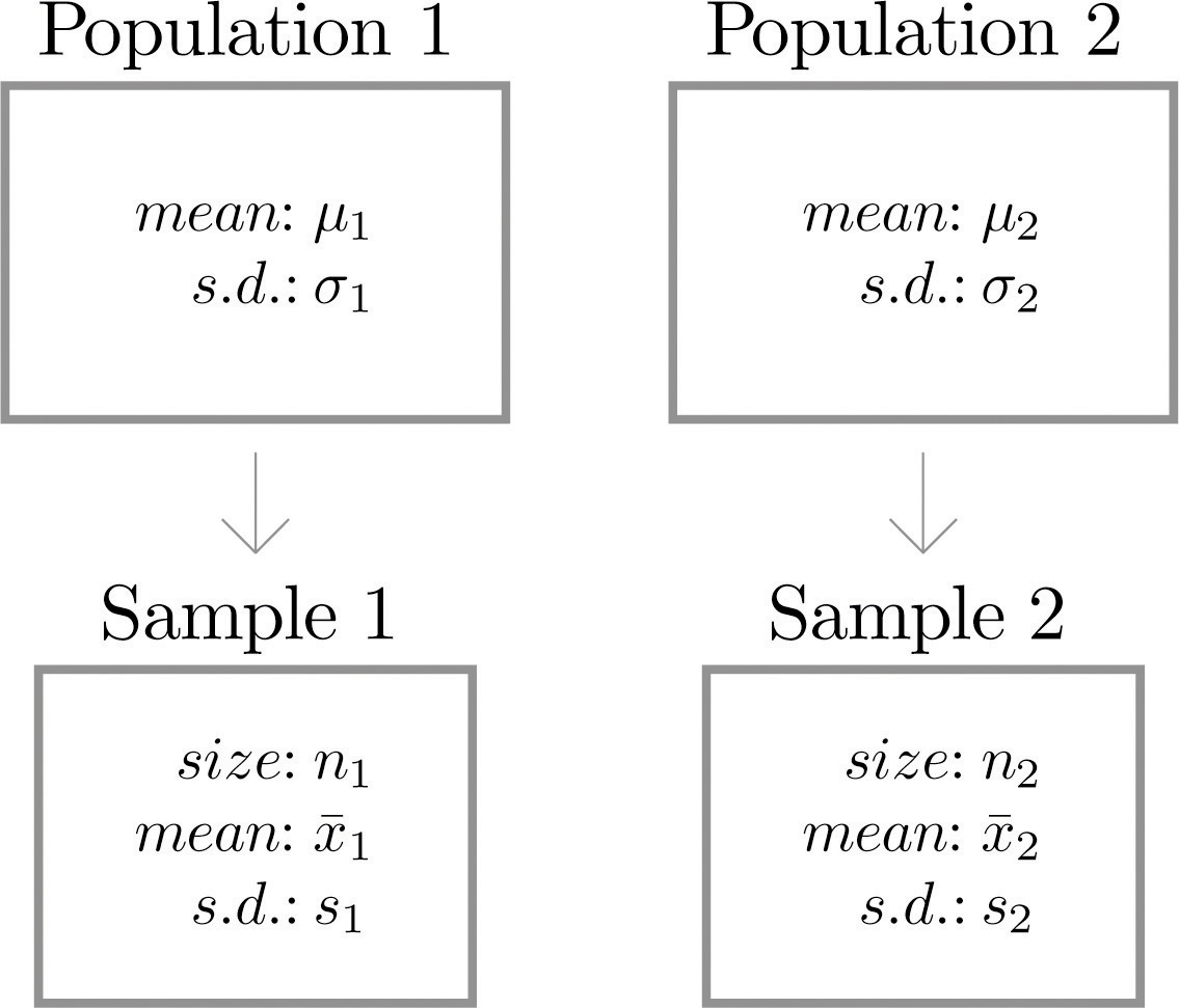
Suppose we wish to compare the means of two distinct populations. Figure 9.1 "Independent Sampling from Two Populations" illustrates the conceptual framework of our investigation in this and the next section. Each population has a mean and a standard deviation. We arbitrarily label one population as Population 1 and the other as Population 2, and subscript the parameters with the numbers 1 and 2 to tell them apart. We draw a random sample from Population 1 and label the sample statistics it yields with the subscript 1. Without reference to the first sample we draw a sample from Population 2 and label its sample statistics with the subscript 2.
Figure 9.1 Independent Sampling from Two Populations
Definition
Samples from two distinct populations are independent if each one is drawn without reference to the other, and has no connection with the other.
Our goal is to use the information in the samples to estimate the difference in the means of the two populations and to make statistically valid inferences about it.
Confidence Intervals
Since the mean of the sample drawn from Population 1 is a good estimator of and the mean of the sample drawn from Population 2 is a good estimator of , a reasonable point estimate of the difference is In order to widen this point estimate into a confidence interval, we first suppose that both samples are large, that is, that both and If so, then the following formula for a confidence interval for is valid. The symbols and denote the squares of s1 and s2. (In the relatively rare case that both population standard deviations and are known they would be used instead of the sample standard deviations.)
Confidence Interval for the Difference Between Two Population Means: Large, Independent Samples
The samples must be independent, and each sample must be large: and
Example 1
To compare customer satisfaction levels of two competing cable television companies, 174 customers of Company 1 and 355 customers of Company 2 were randomly selected and were asked to rate their cable companies on a five-point scale, with 1 being least satisfied and 5 most satisfied. The survey results are summarized in the following table:
| Company 1 | Company 2 |
|---|---|
Construct a point estimate and a 99% confidence interval for , the difference in average satisfaction levels of customers of the two companies as measured on this five-point scale.
Solution:
The point estimate of is
In words, we estimate that the average customer satisfaction level for Company 1 is 0.27 points higher on this five-point scale than it is for Company 2.
To apply the formula for the confidence interval, proceed exactly as was done in Chapter 7 "Estimation". The 99% confidence level means that so that From Figure 12.3 "Critical Values of " we read directly that Thus
We are 99% confident that the difference in the population means lies in the interval , in the sense that in repeated sampling 99% of all intervals constructed from the sample data in this manner will contain In the context of the problem we say we are 99% confident that the average level of customer satisfaction for Company 1 is between 0.15 and 0.39 points higher, on this five-point scale, than that for Company 2.
Hypothesis Testing
Hypotheses concerning the relative sizes of the means of two populations are tested using the same critical value and p-value procedures that were used in the case of a single population. All that is needed is to know how to express the null and alternative hypotheses and to know the formula for the standardized test statistic and the distribution that it follows.
The null and alternative hypotheses will always be expressed in terms of the difference of the two population means. Thus the null hypothesis will always be written
where D0 is a number that is deduced from the statement of the situation. As was the case with a single population the alternative hypothesis can take one of the three forms, with the same terminology:
| Form of | Terminology |
|---|---|
| Left-tailed | |
| Right-tailed | |
| Two-tailed |
As long as the samples are independent and both are large the following formula for the standardized test statistic is valid, and it has the standard normal distribution. (In the relatively rare case that both population standard deviations and are known they would be used instead of the sample standard deviations.)
Standardized Test Statistic for Hypothesis Tests Concerning the Difference Between Two Population Means: Large, Independent Samples
The test statistic has the standard normal distribution.
The samples must be independent, and each sample must be large: and
Example 2
Refer to Note 9.4 "Example 1" concerning the mean satisfaction levels of customers of two competing cable television companies. Test at the 1% level of significance whether the data provide sufficient evidence to conclude that Company 1 has a higher mean satisfaction rating than does Company 2. Use the critical value approach.
Solution:
-
Step 1. If the mean satisfaction levels and are the same then , but we always express the null hypothesis in terms of the difference between and , hence H0 is To say that the mean customer satisfaction for Company 1 is higher than that for Company 2 means that , which in terms of their difference is The test is therefore
-
Step 2. Since the samples are independent and both are large the test statistic is
-
Step 3. Inserting the data into the formula for the test statistic gives
-
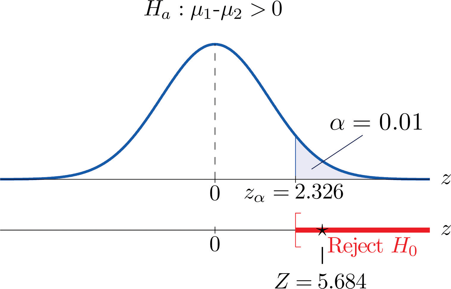
Step 4. Since the symbol in Ha is “>” this is a right-tailed test, so there is a single critical value, , which from the last line in Figure 12.3 "Critical Values of " we read off as 2.326. The rejection region is
Figure 9.2 Rejection Region and Test Statistic for Note 9.6 "Example 2"
-
Step 5. As shown in Figure 9.2 "Rejection Region and Test Statistic for " the test statistic falls in the rejection region. The decision is to reject H0. In the context of the problem our conclusion is:
The data provide sufficient evidence, at the 1% level of significance, to conclude that the mean customer satisfaction for Company 1 is higher than that for Company 2.
Example 3
Perform the test of Note 9.6 "Example 2" using the p-value approach.
Solution:
The first three steps are identical to those in Note 9.6 "Example 2".
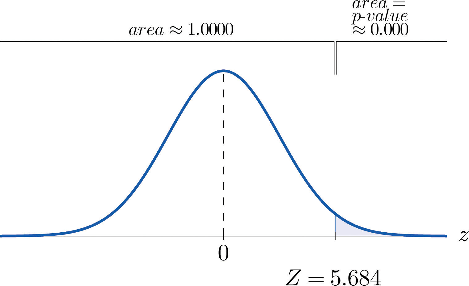
- Step 4. The observed significance or p-value of the test is the area of the right tail of the standard normal distribution that is cut off by the test statistic Z = 5.684. The number 5.684 is too large to appear in Figure 12.2 "Cumulative Normal Probability", which means that the area of the left tail that it cuts off is 1.0000 to four decimal places. The area that we seek, the area of the right tail, is therefore to four decimal places. See Figure 9.3. That is, to four decimal places. (The actual value is approximately )
Figure 9.3 P-Value for Note 9.7 "Example 3"
-
Step 5. Since 0.0000 < 0.01, so the decision is to reject the null hypothesis:
The data provide sufficient evidence, at the 1% level of significance, to conclude that the mean customer satisfaction for Company 1 is higher than that for Company 2.
Key Takeaways
- A point estimate for the difference in two population means is simply the difference in the corresponding sample means.
- In the context of estimating or testing hypotheses concerning two population means, “large” samples means that both samples are large.
- A confidence interval for the difference in two population means is computed using a formula in the same fashion as was done for a single population mean.
- The same five-step procedure used to test hypotheses concerning a single population mean is used to test hypotheses concerning the difference between two population means. The only difference is in the formula for the standardized test statistic.
Exercises
-
Construct the confidence interval for for the level of confidence and the data from independent samples given.
-
90% confidence,
, ,
, ,
-
99% confidence,
, ,
, ,
-
-
Construct the confidence interval for for the level of confidence and the data from independent samples given.
-
95% confidence,
, ,
, ,
-
90% confidence,
, ,
, ,
-
-
Construct the confidence interval for for the level of confidence and the data from independent samples given.
-
99.5% confidence,
, ,
, ,
-
95% confidence,
, ,
, ,
-
-
Construct the confidence interval for for the level of confidence and the data from independent samples given.
-
99.9% confidence,
, ,
, ,
-
90% confidence,
, ,
, ,
-
-
Perform the test of hypotheses indicated, using the data from independent samples given. Use the critical value approach. Compute the p-value of the test as well.
-
Test vs. @ ,
, ,
, ,
-
Test vs. @ ,
, ,
, ,
-
-
Perform the test of hypotheses indicated, using the data from independent samples given. Use the critical value approach. Compute the p-value of the test as well.
-
Test vs. @ ,
, ,
, ,
-
Test vs. @ ,
, ,
, ,
-
-
Perform the test of hypotheses indicated, using the data from independent samples given. Use the critical value approach. Compute the p-value of the test as well.
-
Test vs. @ ,
, ,
, ,
-
Test vs. @ ,
, ,
, ,
-
-
Perform the test of hypotheses indicated, using the data from independent samples given. Use the critical value approach. Compute the p-value of the test as well.
-
Test vs. @ ,
, ,
, ,
-
Test vs. @ ,
, ,
, ,
-
-
Perform the test of hypotheses indicated, using the data from independent samples given. Use the p-value approach.
-
Test vs. @ ,
, ,
, ,
-
Test vs. @ ,
, ,
, ,
-
-
Perform the test of hypotheses indicated, using the data from independent samples given. Use the p-value approach.
-
Test vs. @ ,
, ,
, ,
-
Test vs. @ ,
, ,
, ,
-
-
Perform the test of hypotheses indicated, using the data from independent samples given. Use the p-value approach.
-
Test vs. @ ,
, ,
, ,
-
Test vs. @ ,
, ,
, ,
-
-
Perform the test of hypotheses indicated, using the data from independent samples given. Use the p-value approach.
-
Test vs. @ ,
, ,
, ,
-
Test vs. @ ,
, ,
, ,
-
Basic
-
In order to investigate the relationship between mean job tenure in years among workers who have a bachelor’s degree or higher and those who do not, random samples of each type of worker were taken, with the following results.
n s Bachelor’s degree or higher 155 5.2 1.3 No degree 210 5.0 1.5 - Construct the 99% confidence interval for the difference in the population means based on these data.
- Test, at the 1% level of significance, the claim that mean job tenure among those with higher education is greater than among those without, against the default that there is no difference in the means.
- Compute the observed significance of the test.
-
Records of 40 used passenger cars and 40 used pickup trucks (none used commercially) were randomly selected to investigate whether there was any difference in the mean time in years that they were kept by the original owner before being sold. For cars the mean was 5.3 years with standard deviation 2.2 years. For pickup trucks the mean was 7.1 years with standard deviation 3.0 years.
- Construct the 95% confidence interval for the difference in the means based on these data.
- Test the hypothesis that there is a difference in the means against the null hypothesis that there is no difference. Use the 1% level of significance.
- Compute the observed significance of the test in part (b).
-
In previous years the average number of patients per hour at a hospital emergency room on weekends exceeded the average on weekdays by 6.3 visits per hour. A hospital administrator believes that the current weekend mean exceeds the weekday mean by fewer than 6.3 hours.
-
Construct the 99% confidence interval for the difference in the population means based on the following data, derived from a study in which 30 weekend and 30 weekday one-hour periods were randomly selected and the number of new patients in each recorded.
n s Weekends 30 13.8 3.1 Weekdays 30 8.6 2.7 - Test at the 5% level of significance whether the current weekend mean exceeds the weekday mean by fewer than 6.3 patients per hour.
- Compute the observed significance of the test.
-
-
A sociologist surveys 50 randomly selected citizens in each of two countries to compare the mean number of hours of volunteer work done by adults in each. Among the 50 inhabitants of Lilliput, the mean hours of volunteer work per year was 52, with standard deviation 11.8. Among the 50 inhabitants of Blefuscu, the mean number of hours of volunteer work per year was 37, with standard deviation 7.2.
- Construct the 99% confidence interval for the difference in mean number of hours volunteered by all residents of Lilliput and the mean number of hours volunteered by all residents of Blefuscu.
- Test, at the 1% level of significance, the claim that the mean number of hours volunteered by all residents of Lilliput is more than ten hours greater than the mean number of hours volunteered by all residents of Blefuscu.
- Compute the observed significance of the test in part (b).
-
A university administrator asserted that upperclassmen spend more time studying than underclassmen.
-
Test this claim against the default that the average number of hours of study per week by the two groups is the same, using the following information based on random samples from each group of students. Test at the 1% level of significance.
n s Upperclassmen 35 15.6 2.9 Underclassmen 35 12.3 4.1 - Compute the observed significance of the test.
-
-
An kinesiologist claims that the resting heart rate of men aged 18 to 25 who exercise regularly is more than five beats per minute less than that of men who do not exercise regularly. Men in each category were selected at random and their resting heart rates were measured, with the results shown.
n s Regular exercise 40 63 1.0 No regular exercise 30 71 1.2 - Perform the relevant test of hypotheses at the 1% level of significance.
- Compute the observed significance of the test.
-
Children in two elementary school classrooms were given two versions of the same test, but with the order of questions arranged from easier to more difficult in Version A and in reverse order in Version B. Randomly selected students from each class were given Version A and the rest Version B. The results are shown in the table.
n s Version A 31 83 4.6 Version B 32 78 4.3 - Construct the 90% confidence interval for the difference in the means of the populations of all children taking Version A of such a test and of all children taking Version B of such a test.
- Test at the 1% level of significance the hypothesis that the A version of the test is easier than the B version (even though the questions are the same).
- Compute the observed significance of the test.
-
The Municipal Transit Authority wants to know if, on weekdays, more passengers ride the northbound blue line train towards the city center that departs at 8:15 a.m. or the one that departs at 8:30 a.m. The following sample statistics are assembled by the Transit Authority.
n s 8:15 a.m. train 30 323 41 8:30 a.m. train 45 356 45 - Construct the 90% confidence interval for the difference in the mean number of daily travellers on the 8:15 train and the mean number of daily travellers on the 8:30 train.
- Test at the 5% level of significance whether the data provide sufficient evidence to conclude that more passengers ride the 8:30 train.
- Compute the observed significance of the test.
-
In comparing the academic performance of college students who are affiliated with fraternities and those male students who are unaffiliated, a random sample of students was drawn from each of the two populations on a university campus. Summary statistics on the student GPAs are given below.
n s Fraternity 645 2.90 0.47 Unaffiliated 450 2.88 0.42 Test, at the 5% level of significance, whether the data provide sufficient evidence to conclude that there is a difference in average GPA between the population of fraternity students and the population of unaffiliated male students on this university campus.
-
In comparing the academic performance of college students who are affiliated with sororities and those female students who are unaffiliated, a random sample of students was drawn from each of the two populations on a university campus. Summary statistics on the student GPAs are given below.
n s Sorority 330 3.18 0.37 Unaffiliated 550 3.12 0.41 Test, at the 5% level of significance, whether the data provide sufficient evidence to conclude that there is a difference in average GPA between the population of sorority students and the population of unaffiliated female students on this university campus.
-
The owner of a professional football team believes that the league has become more offense oriented since five years ago. To check his belief, 32 randomly selected games from one year’s schedule were compared to 32 randomly selected games from the schedule five years later. Since more offense produces more points per game, the owner analyzed the following information on points per game (ppg).
n s ppg previously 32 20.62 4.17 ppg recently 32 22.05 4.01 Test, at the 10% level of significance, whether the data on points per game provide sufficient evidence to conclude that the game has become more offense oriented.
-
The owner of a professional football team believes that the league has become more offense oriented since five years ago. To check his belief, 32 randomly selected games from one year’s schedule were compared to 32 randomly selected games from the schedule five years later. Since more offense produces more offensive yards per game, the owner analyzed the following information on offensive yards per game (oypg).
n s oypg previously 32 316 40 oypg recently 32 336 35 Test, at the 10% level of significance, whether the data on offensive yards per game provide sufficient evidence to conclude that the game has become more offense oriented.
Applications
-
Large Data Sets 1A and 1B list the SAT scores for 1,000 randomly selected students. Denote the population of all male students as Population 1 and the population of all female students as Population 2.
http://www.flatworldknowledge.com/sites/all/files/data1A.xls
http://www.flatworldknowledge.com/sites/all/files/data1B.xls
- Restricting attention to just the males, find n1, , and s1. Restricting attention to just the females, find n2, , and s2.
- Let denote the mean SAT score for all males and the mean SAT score for all females. Use the results of part (a) to construct a 90% confidence interval for the difference
- Test, at the 5% level of significance, the hypothesis that the mean SAT scores among males exceeds that of females.
-
Large Data Sets 1A and 1B list the GPAs for 1,000 randomly selected students. Denote the population of all male students as Population 1 and the population of all female students as Population 2.
http://www.flatworldknowledge.com/sites/all/files/data1A.xls
http://www.flatworldknowledge.com/sites/all/files/data1B.xls
- Restricting attention to just the males, find n1, , and s1. Restricting attention to just the females, find n2, , and s2.
- Let denote the mean GPA for all males and the mean GPA for all females. Use the results of part (a) to construct a 95% confidence interval for the difference
- Test, at the 10% level of significance, the hypothesis that the mean GPAs among males and females differ.
-
Large Data Sets 7A and 7B list the survival times for 65 male and 75 female laboratory mice with thymic leukemia. Denote the population of all such male mice as Population 1 and the population of all such female mice as Population 2.
http://www.flatworldknowledge.com/sites/all/files/data7A.xls
http://www.flatworldknowledge.com/sites/all/files/data7B.xls
- Restricting attention to just the males, find n1, , and s1. Restricting attention to just the females, find n2, , and s2.
- Let denote the mean survival for all males and the mean survival time for all females. Use the results of part (a) to construct a 99% confidence interval for the difference
- Test, at the 1% level of significance, the hypothesis that the mean survival time for males exceeds that for females by more than 182 days (half a year).
- Compute the observed significance of the test in part (c).
Large Data Set Exercises
Answers
-
- ,
-
-
- ,
-
-
- Z = 8.753, , reject H0, p-value = 0.0000;
- , , do not reject H0, p-value = 0.2451
-
-
- Z = 2.444, , do not reject H0, p-value = 0.0146.
- Z = 1.702, , reject H0, p-value = 0.0446
-
-
- , p-value = 0.1170, do not reject H0;
- , p-value = 0.3576, do not reject H0
-
-
- Z = 2.68, p-value = 0.0037, reject H0;
- , p-value = 0.1802, do not reject H0
-
-
- ,
- Z = 1.360, , do not reject H0 (not greater)
- p-value = 0.0869
-
-
- ,
- , , do not reject H0 (exceeds by 6.3 or more)
- p-value = 0.0708
-
-
- Z = 3.888, , reject H0 (upperclassmen study more)
- p-value = 0.0001
-
-
- ,
- Z = 4.454, , reject H0 (Test A is easier)
- p-value = 0.0000
-
-
Z = 0.738, , do not reject H0 (no difference)
-
-
, , reject H0 (more offense oriented)
-
-
- , , , , , and
- vs. Test Statistic: Z = 1.48. Rejection Region: Decision: Fail to reject H0.
-
-
- , , , , , and
- vs. Test Statistic: Z = 3.14. Rejection Region: Decision: Reject H0.