This is “Areas of Tails of Distributions”, section 5.4 from the book Beginning Statistics (v. 1.0). For details on it (including licensing), click here.
For more information on the source of this book, or why it is available for free, please see the project's home page. You can browse or download additional books there. To download a .zip file containing this book to use offline, simply click here.


5.4 Areas of Tails of Distributions
Learning Objective
- To learn how to find, for a normal random variable X and an area a, the value of X so that or that , whichever is required.
Definition
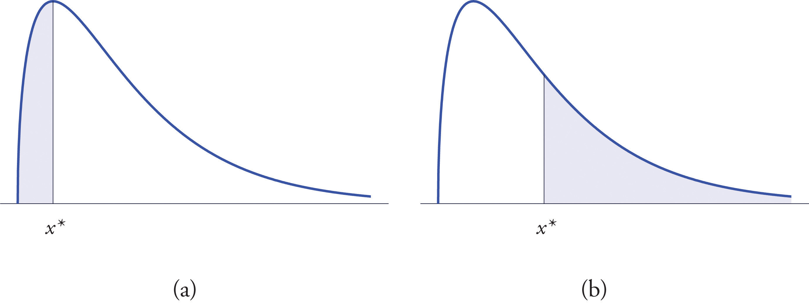
The left tailThe region under a density curve whose area is either or for some number . of a density curve of a continuous random variable X cut off by a value of X is the region under the curve that is to the left of , as shown by the shading in Figure 5.19 "Right and Left Tails of a Distribution"(a). The right tail cut off by is defined similarly, as indicated by the shading in Figure 5.19 "Right and Left Tails of a Distribution"(b).
Figure 5.19 Right and Left Tails of a Distribution
The probabilities tabulated in Figure 12.2 "Cumulative Normal Probability" are areas of left tails in the standard normal distribution.
Tails of the Standard Normal Distribution
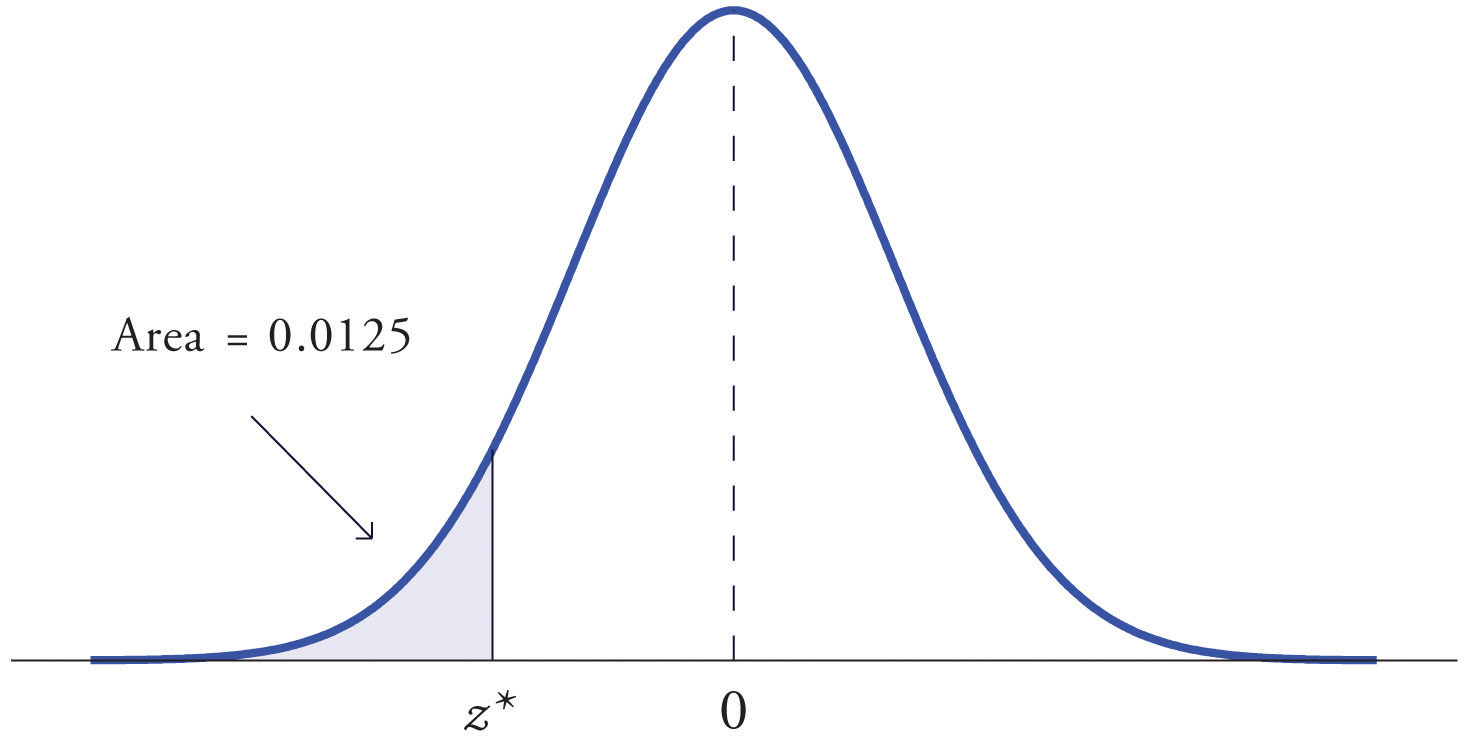
At times it is important to be able to solve the kind of problem illustrated by Figure 5.20. We have a certain specific area in mind, in this case the area 0.0125 of the shaded region in the figure, and we want to find the value of Z that produces it. This is exactly the reverse of the kind of problems encountered so far. Instead of knowing a value of Z and finding a corresponding area, we know the area and want to find In the case at hand, in the terminology of the definition just above, we wish to find the value that cuts off a left tail of area 0.0125 in the standard normal distribution.
The idea for solving such a problem is fairly simple, although sometimes its implementation can be a bit complicated. In a nutshell, one reads the cumulative probability table for Z in reverse, looking up the relevant area in the interior of the table and reading off the value of Z from the margins.
Figure 5.20 Z Value that Produces a Known Area
Example 12
Find the value of Z as determined by Figure 5.20: the value that cuts off a left tail of area 0.0125 in the standard normal distribution. In symbols, find the number such that
Solution:
The number that is known, 0.0125, is the area of a left tail, and as already mentioned the probabilities tabulated in Figure 12.2 "Cumulative Normal Probability" are areas of left tails. Thus to solve this problem we need only search in the interior of Figure 12.2 "Cumulative Normal Probability" for the number 0.0125. It lies in the row with the heading −2.2 and in the column with the heading 0.04. This means that P(Z < −2.24) = 0.0125, hence
Example 13
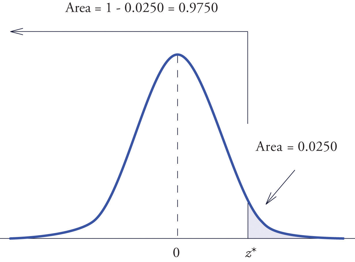
Find the value of Z as determined by Figure 5.21: the value that cuts off a right tail of area 0.0250 in the standard normal distribution. In symbols, find the number such that
Figure 5.21 Z Value that Produces a Known Area
Solution:
The important distinction between this example and the previous one is that here it is the area of a right tail that is known. In order to be able to use Figure 12.2 "Cumulative Normal Probability" we must first find that area of the left tail cut off by the unknown number Since the total area under the density curve is 1, that area is This is the number we look for in the interior of Figure 12.2 "Cumulative Normal Probability". It lies in the row with the heading 1.9 and in the column with the heading 0.06. Therefore
Definition
The value of the standard normal random variable Z that cuts off a right tail of area c is denoted zc. By symmetry, value of Z that cuts off a left tail of area c is See Figure 5.22 "The Numbers ".
Figure 5.22 The Numbers zc and

The previous two examples were atypical because the areas we were looking for in the interior of Figure 12.2 "Cumulative Normal Probability" were actually there. The following example illustrates the situation that is more common.
Example 14
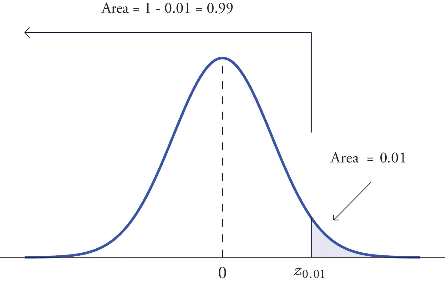
Find and , the values of Z that cut off right and left tails of area 0.01 in the standard normal distribution.
Solution:
Since cuts off a left tail of area 0.01 and Figure 12.2 "Cumulative Normal Probability" is a table of left tails, we look for the number 0.0100 in the interior of the table. It is not there, but falls between the two numbers 0.0102 and 0.0099 in the row with heading −2.3. The number 0.0099 is closer to 0.0100 than 0.0102 is, so for the hundredths place in we use the heading of the column that contains 0.0099, namely, 0.03, and write
The answer to the second half of the problem is automatic: since , we conclude immediately that
We could just as well have solved this problem by looking for first, and it is instructive to rework the problem this way. To begin with, we must first subtract 0.01 from 1 to find the area of the left tail cut off by the unknown number See Figure 5.23 "Computation of the Number ". Then we search for the area 0.9900 in Figure 12.2 "Cumulative Normal Probability". It is not there, but falls between the numbers 0.9898 and 0.9901 in the row with heading 2.3. Since 0.9901 is closer to 0.9900 than 0.9898 is, we use the column heading above it, 0.03, to obtain the approximation Then finally
Figure 5.23 Computation of the Number
Tails of General Normal Distributions
The problem of finding the value of a general normally distributed random variable X that cuts off a tail of a specified area also arises. This problem may be solved in two steps.
Suppose X is a normally distributed random variable with mean μ and standard deviation σ. To find the value of X that cuts off a left or right tail of area c in the distribution of X:
- find the value of Z that cuts off a left or right tail of area c in the standard normal distribution;
-
is the z-score of ; compute using the destandardization formula
In short, solve the corresponding problem for the standard normal distribution, thereby obtaining the z-score of , then destandardize to obtain
Example 15
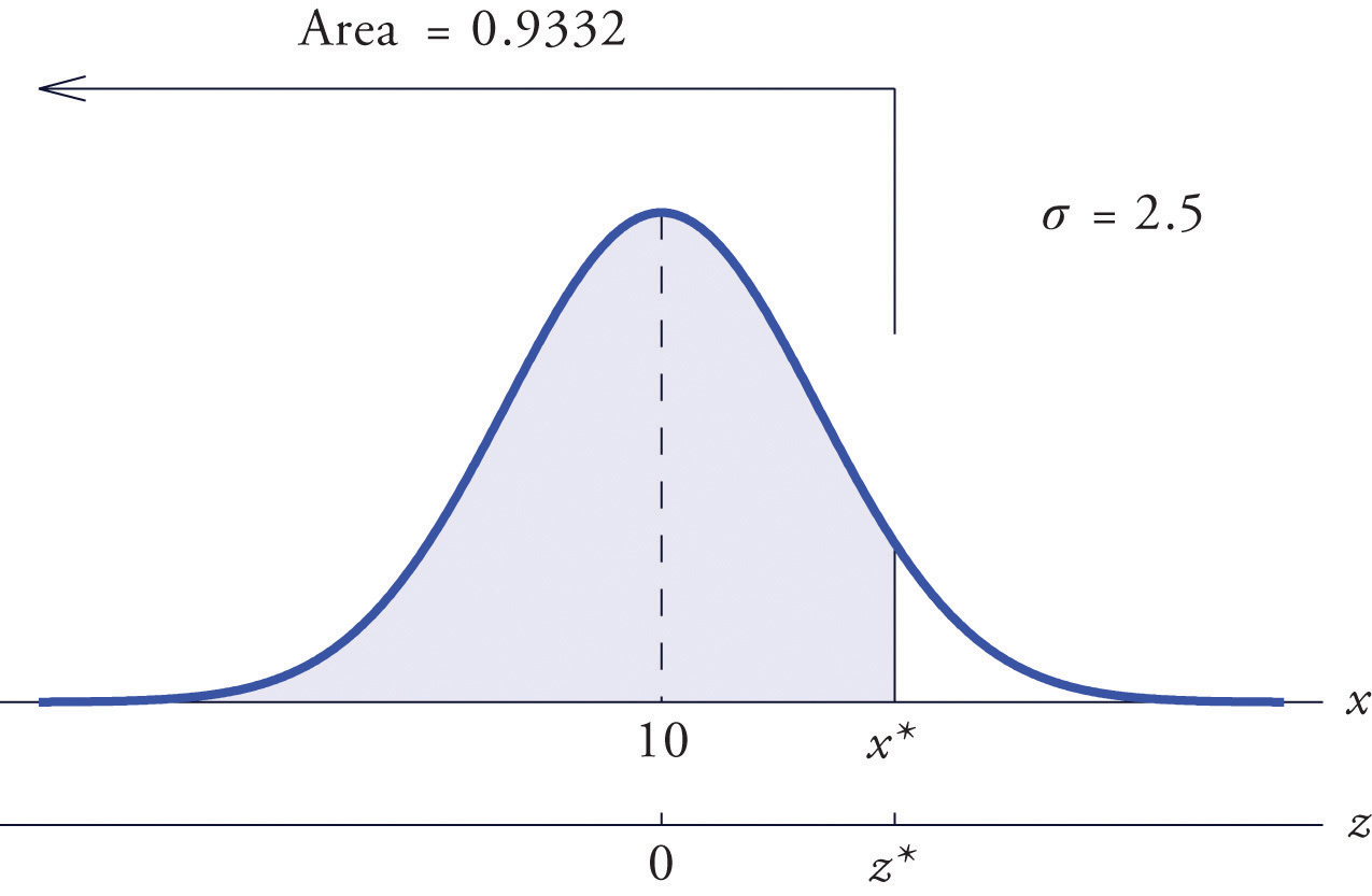
Find such that , where X is a normal random variable with mean μ = 10 and standard deviation σ = 2.5.
Solution:
All the ideas for the solution are illustrated in Figure 5.24 "Tail of a Normally Distributed Random Variable". Since 0.9332 is the area of a left tail, we can find simply by looking for 0.9332 in the interior of Figure 12.2 "Cumulative Normal Probability". It is in the row and column with headings 1.5 and 0.00, hence Thus is 1.50 standard deviations above the mean, so
Figure 5.24 Tail of a Normally Distributed Random Variable
Example 16
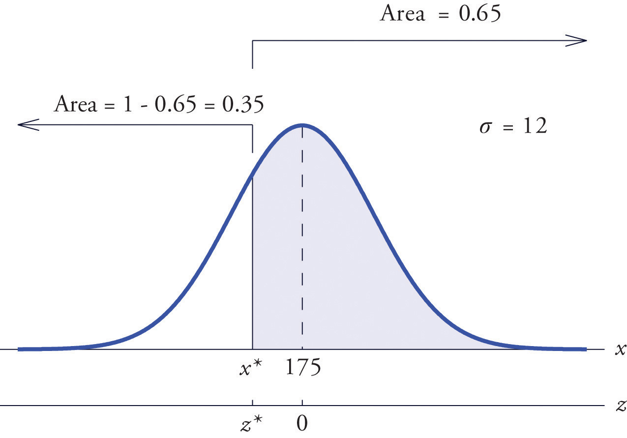
Find such that , where X is a normal random variable with mean μ = 175 and standard deviation σ = 12.
Solution:
The situation is illustrated in Figure 5.25 "Tail of a Normally Distributed Random Variable". Since 0.65 is the area of a right tail, we first subtract it from 1 to obtain , the area of the complementary left tail. We find by looking for 0.3500 in the interior of Figure 12.2 "Cumulative Normal Probability". It is not present, but lies between table entries 0.3520 and 0.3483. The entry 0.3483 with row and column headings −0.3 and 0.09 is closer to 0.3500 than the other entry is, so Thus is 0.39 standard deviations below the mean, so
Figure 5.25 Tail of a Normally Distributed Random Variable
Example 17
Scores on a standardized college entrance examination (CEE) are normally distributed with mean 510 and standard deviation 60. A selective university decides to give serious consideration for admission to applicants whose CEE scores are in the top 5% of all CEE scores. Find the minimum score that meets this criterion for serious consideration for admission.
Solution:
Let X denote the score made on the CEE by a randomly selected individual. Then X is normally distributed with mean 510 and standard deviation 60. The probability that X lie in a particular interval is the same as the proportion of all exam scores that lie in that interval. Thus the minimum score that is in the top 5% of all CEE is the score that cuts off a right tail in the distribution of X of area 0.05 (5% expressed as a proportion). See Figure 5.26 "Tail of a Normally Distributed Random Variable".
Figure 5.26 Tail of a Normally Distributed Random Variable
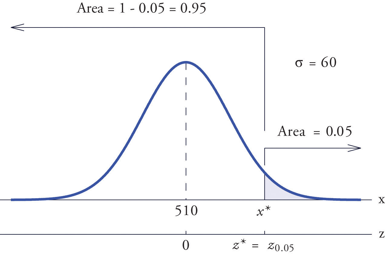
Since 0.0500 is the area of a right tail, we first subtract it from 1 to obtain , the area of the complementary left tail. We find by looking for 0.9500 in the interior of Figure 12.2 "Cumulative Normal Probability". It is not present, and lies exactly half-way between the two nearest entries that are, 0.9495 and 0.9505. In the case of a tie like this, we will always average the values of Z corresponding to the two table entries, obtaining here the value Using this value, we conclude that is 1.645 standard deviations above the mean, so
Example 18
All boys at a military school must run a fixed course as fast as they can as part of a physical examination. Finishing times are normally distributed with mean 29 minutes and standard deviation 2 minutes. The middle 75% of all finishing times are classified as “average.” Find the range of times that are average finishing times by this definition.
Solution:
Let X denote the finish time of a randomly selected boy. Then X is normally distributed with mean 29 and standard deviation 2. The probability that X lie in a particular interval is the same as the proportion of all finish times that lie in that interval. Thus the situation is as shown in Figure 5.27 "Distribution of Times to Run a Course". Because the area in the middle corresponding to “average” times is 0.75, the areas of the two tails add up to 1 − 0.75 = 0.25 in all. By the symmetry of the density curve each tail must have half of this total, or area 0.125 each. Thus the fastest time that is “average” has z-score , which by Figure 12.2 "Cumulative Normal Probability" is −1.15, and the slowest time that is “average” has z-score The fastest and slowest times that are still considered average are
and
Figure 5.27 Distribution of Times to Run a Course
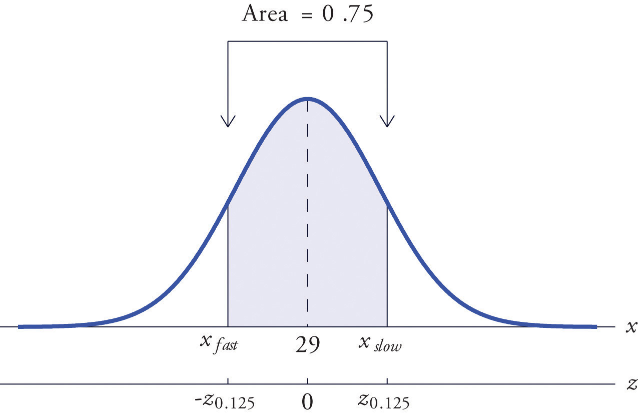
A boy has an average finishing time if he runs the course with a time between 26.7 and 31.3 minutes, or equivalently between 26 minutes 42 seconds and 31 minutes 18 seconds.
Key Takeaways
- The problem of finding the number so that the probability is a specified value c is solved by looking for the number c in the interior of Figure 12.2 "Cumulative Normal Probability" and reading from the margins.
- The problem of finding the number so that the probability is a specified value c is solved by looking for the complementary probability in the interior of Figure 12.2 "Cumulative Normal Probability" and reading from the margins.
- For a normal random variable X with mean μ and standard deviation σ, the problem of finding the number so that is a specified value c (or so that is a specified value c) is solved in two steps: (1) solve the corresponding problem for Z with the same value of c, thereby obtaining the z-score, , of ; (2) find using
- The value of Z that cuts off a right tail of area c in the standard normal distribution is denoted zc.
Exercises
-
Find the value of that yields the probability shown.
-
Find the value of that yields the probability shown.
-
Find the value of that yields the probability shown.
-
Find the value of that yields the probability shown.
-
Find the indicated value of Z. (It is easier to find and negate it.)
- z0.025
- z0.20
-
Find the indicated value of Z. (It is easier to find and negate it.)
- z0.002
- z0.02
-
Find the value of that yields the probability shown, where X is a normally distributed random variable X with mean 83 and standard deviation 4.
-
Find the value of that yields the probability shown, where X is a normally distributed random variable X with mean 54 and standard deviation 12.
-
X is a normally distributed random variable X with mean 15 and standard deviation 0.25. Find the values xL and xR of X that are symmetrically located with respect to the mean of X and satisfy P(xL < X < xR) = 0.80. (Hint. First solve the corresponding problem for Z.)
-
X is a normally distributed random variable X with mean 28 and standard deviation 3.7. Find the values xL and xR of X that are symmetrically located with respect to the mean of X and satisfy P(xL < X < xR) = 0.65. (Hint. First solve the corresponding problem for Z.)
Basic
-
Scores on a national exam are normally distributed with mean 382 and standard deviation 26.
- Find the score that is the 50th percentile.
- Find the score that is the 90th percentile.
-
Heights of women are normally distributed with mean 63.7 inches and standard deviation 2.47 inches.
- Find the height that is the 10th percentile.
- Find the height that is the 80th percentile.
-
The monthly amount of water used per household in a small community is normally distributed with mean 7,069 gallons and standard deviation 58 gallons. Find the three quartiles for the amount of water used.
-
The quantity of gasoline purchased in a single sale at a chain of filling stations in a certain region is normally distributed with mean 11.6 gallons and standard deviation 2.78 gallons. Find the three quartiles for the quantity of gasoline purchased in a single sale.
-
Scores on the common final exam given in a large enrollment multiple section course were normally distributed with mean 69.35 and standard deviation 12.93. The department has the rule that in order to receive an A in the course his score must be in the top 10% of all exam scores. Find the minimum exam score that meets this requirement.
-
The average finishing time among all high school boys in a particular track event in a certain state is 5 minutes 17 seconds. Times are normally distributed with standard deviation 12 seconds.
- The qualifying time in this event for participation in the state meet is to be set so that only the fastest 5% of all runners qualify. Find the qualifying time. (Hint: Convert seconds to minutes.)
- In the western region of the state the times of all boys running in this event are normally distributed with standard deviation 12 seconds, but with mean 5 minutes 22 seconds. Find the proportion of boys from this region who qualify to run in this event in the state meet.
-
Tests of a new tire developed by a tire manufacturer led to an estimated mean tread life of 67,350 miles and standard deviation of 1,120 miles. The manufacturer will advertise the lifetime of the tire (for example, a “50,000 mile tire”) using the largest value for which it is expected that 98% of the tires will last at least that long. Assuming tire life is normally distributed, find that advertised value.
-
Tests of a new light led to an estimated mean life of 1,321 hours and standard deviation of 106 hours. The manufacturer will advertise the lifetime of the bulb using the largest value for which it is expected that 90% of the bulbs will last at least that long. Assuming bulb life is normally distributed, find that advertised value.
-
The weights X of eggs produced at a particular farm are normally distributed with mean 1.72 ounces and standard deviation 0.12 ounce. Eggs whose weights lie in the middle 75% of the distribution of weights of all eggs are classified as “medium.” Find the maximum and minimum weights of such eggs. (These weights are endpoints of an interval that is symmetric about the mean and in which the weights of 75% of the eggs produced at this farm lie.)
-
The lengths X of hardwood flooring strips are normally distributed with mean 28.9 inches and standard deviation 6.12 inches. Strips whose lengths lie in the middle 80% of the distribution of lengths of all strips are classified as “average-length strips.” Find the maximum and minimum lengths of such strips. (These lengths are endpoints of an interval that is symmetric about the mean and in which the lengths of 80% of the hardwood strips lie.)
-
All students in a large enrollment multiple section course take common in-class exams and a common final, and submit common homework assignments. Course grades are assigned based on students' final overall scores, which are approximately normally distributed. The department assigns a C to students whose scores constitute the middle 2/3 of all scores. If scores this semester had mean 72.5 and standard deviation 6.14, find the interval of scores that will be assigned a C.
-
Researchers wish to investigate the overall health of individuals with abnormally high or low levels of glucose in the blood stream. Suppose glucose levels are normally distributed with mean 96 and standard deviation 8.5 mg/d , and that “normal” is defined as the middle 90% of the population. Find the interval of normal glucose levels, that is, the interval centered at 96 that contains 90% of all glucose levels in the population.
Applications
-
A machine for filling 2-liter bottles of soft drink delivers an amount to each bottle that varies from bottle to bottle according to a normal distribution with standard deviation 0.002 liter and mean whatever amount the machine is set to deliver.
- If the machine is set to deliver 2 liters (so the mean amount delivered is 2 liters) what proportion of the bottles will contain at least 2 liters of soft drink?
- Find the minimum setting of the mean amount delivered by the machine so that at least 99% of all bottles will contain at least 2 liters.
-
A nursery has observed that the mean number of days it must darken the environment of a species poinsettia plant daily in order to have it ready for market is 71 days. Suppose the lengths of such periods of darkening are normally distributed with standard deviation 2 days. Find the number of days in advance of the projected delivery dates of the plants to market that the nursery must begin the daily darkening process in order that at least 95% of the plants will be ready on time. (Poinsettias are so long-lived that once ready for market the plant remains salable indefinitely.)
Additional Exercises
Answers
-
- −2.43
- 2.17
- −1.28
- 2.29
-
-
- −1.04
- 0.67
- 0.43
- −0.84
-
-
- 1.96
- 0.84
-
-
- 87.52
- 89.58
-
-
15.32
-
-
- 382
- 415
-
-
7030.14, 7069, 7107.86
-
-
85.90
-
-
65,054
-
-
1.58, 1.86
-
-
66.5, 78.5
-
-
- 0.5
- 2.005
-