This is “Chapter Assignments and Tests”, section 2.4 from the book Using Microsoft Excel (v. 1.1). For details on it (including licensing), click here.
For more information on the source of this book, or why it is available for free, please see the project's home page. You can browse or download additional books there. To download a .zip file containing this book to use offline, simply click here.


2.4 Chapter Assignments and Tests
To assess your understanding of the material covered in the chapter, please complete the following assignments.
Careers in Practice (Skills Review)
Financial Plan for a Lawn Care Business (Comprehensive Review)
Starter File: Chapter 2 CiP Exercise 1
Difficulty: Level 1 Easy
Running your own lawn care business can be an excellent way to make money over the summer while on break from college. It can also be a way to supplement your existing income for the purpose of saving money for retirement or for a college fund. However, managing the costs of the business will be critical in order for it to be a profitable venture. In this exercise you will create a simple financial plan for a lawn care business by using the skills covered in this chapter. Begin this exercise by opening the file named Chapter 2 CiP Exercise 1.
- Click cell C5 in the Annual Plan worksheet.
- Enter a formula that calculates the average price per lawn cut. Type an equal sign (=), then click cell B3. Type the asterisk symbol (*) for multiplication, then click cell B4. Press the ENTER key.
- Click cell C8 in the Annual Plan worksheet.
- Enter a formula that calculates the total number of lawns that will be cut during the year. Type an equal sign (=), then click cell B6. Type the asterisk symbol (*) for multiplication, then click cell B7. Press the ENTER key.
- Click cell D9 in the Annual Plan worksheet.
- Enter a formula that calculates the total sales for the plan. Type an equal sign (=), then click cell C5. Type the asterisk symbol (*) for multiplication, then click cell C8. Press the ENTER key.
- Click cell F3 in the Leases worksheet. The PMT function will be used to calculate the monthly lease payment for the first item. For many businesses, leasing (or renting) equipment is a more favorable option than purchasing equipment because it requires far less cash. This enables you to begin a business such as a lawn care business without having to put up a lot of money to buy equipment.
-
Type an equal sign (=) followed by the function name PMT and an open parenthesis ((). Define the arguments of the function as follows:
- Rate: Click cell B3, type a forward slash (/) for division, type the number 12, and type a comma. Since we are calculating monthly payments, the annual interest rate must be converted to a monthly interest rate.
- Nper: Click cell C3, type an asterisk (*) for multiplication, type the number 12, and type a comma. Similar to the Rate argument, the terms of the lease must be converted to months since we are calculating monthly payments.
- Pv: Type a minus sign (−), click cell D3, and type a comma. Remember that this argument must always be preceded by a minus sign.
- Fv: Click cell E3 and type a comma.
- Type: Type the number 1, type a closing parenthesis ()), and press the ENTER key. We will assume the lease payments will be made at the beginning of each month, which requires that this argument be defined with a value of 1.
- Copy the PMT function in cell F3 and paste it into the range F4:F6.
- Click cell F10 in the Leases worksheet. A SUM function will be added to calculate the total for the monthly lease payments.
- Type an equal sign (=) followed by the word SUM and an open parenthesis ((). Highlight the range F3:F9, type a closing parenthesis ()), and press the ENTER key. You will notice that blank rows were included in this range for the SUM function. If other items are added to the worksheet, they will be included in the output of the SUM function.
- Highlight the range A2:F6 on the Leases worksheet. The data in this range will be sorted.
- Click the Sort button in the Data tab of the Ribbon. In the Sort dialog box, select the Interest Rate option in the “Sort by” drop-down box. Select Largest to Smallest for the sort order. Then, click the Add Level button on the Sort dialog box. Select the Price option in the “Then by” drop-down box. Select Largest to Smallest for the sort order. Click the OK button in the Sort dialog box.
- Click cell B11 on the Annual Plan worksheet. The monthly lease payments that are calculated in the Lease worksheet will be displayed in this cell.
- Type an equal sign (=). Click the Leases worksheet tab, click cell F10, and press the ENTER key.
- Click cell C12 on the Annual Plan worksheet.
- Type an equal sign (=) and click cell B11. Type an asterisk (*), type the number 12, and press the ENTER key. This formula calculates the annual lease payments.
- Format the output of the formula in cell C12 so the decimal places are reduced to zero.
- Click cell C14 on the Annual Plan worksheet.
- Type an equal sign (=) and click cell B13. Type an asterisk (*), click cell C8, and press the ENTER key.
- Click cell D16 on the Annual Plan worksheet.
- Type an equal sign (=) followed by the word SUM and an open parenthesis ((). Highlight the range C11:C15, type a closing parenthesis ()), and press the ENTER key. This SUM function adds the total expenses for the business.
- Click cell D17 on the Annual Plan worksheet.
- Type an equal sign (=). Click cell D9, type a minus sign (–), click cell D16, and press the ENTER key. This formula calculates the annual profit for the business.
- Click cell B10 on the Investments worksheet.
- Type an equal sign (=) followed by the word COUNT and an open parenthesis ((). Highlight the range B3:B8, type a closing parenthesis ()), and press the ENTER key. This function counts the number of investments that currently have a balance. Notice that additional blank rows were included in the range for this function. The function output will automatically change if any new investments are added to the worksheet.
- Click cell D3 on the Investments worksheet.
- Type an equal sign (=). Click the Annual Plan worksheet tab. Click cell D17 and type a forward slash (/) for division. Click the Investments worksheet tab. Click cell B10 and press the ENTER key. This formula divides the profit calculated on the Annual Plan worksheet by the number of investments in the Investments worksheet. We will assume that the profits from this business will be invested evenly among the funds listed in Column A of the Investments worksheet.
- Before copying and pasting the formula created in step 28, absolute references must be added to the cell locations in the formula. Double click cell D3 on the Investments worksheet. Place the mouse pointer in front of D17 in the formula and click. Press the F4 key on your keyboard. Place the mouse pointer in front of cell B10 in the formula and click. Press the F4 key on your keyboard. Press the ENTER key.
- Copy cell D3 and paste it into cells D4 and D5.
- Click cell E3 on the Investments worksheet. The future value function will be added to project the total growth of the investments listed in Column A. We will assume that the business will be able to consistently generate the profit, which will be invested evenly in the funds every year.
-
Type an equal sign (=) followed by the function name FV and an open parenthesis ((). Define the arguments of the function as follows:
- Rate: Click cell C3 and type a comma. This is the expected growth rate of the first fund.
- Nper: Type the number 10 and then type a comma. We will project the growth of these investments in 10 years.
- Pmt: Type a minus sign (−), click cell D3, and type a comma. Remember that this argument must always be preceded by a minus sign. We are assuming that the business will consistently generate the profits calculated in the Annual Plan worksheet and that these profits will be invested evenly into each fund.
- Pv: Type a minus sign (–) and click cell B3. Since each fund currently has a balance, we need to add this to the Pv argument of the function. Similar to the Pmt argument, remember that this argument must also be preceded by a minus sign.
- Type: Type a closing parenthesis ()) and press the ENTER key. We will assume the investments will be made at the end of each year. Therefore, it is not necessary to define this argument since Excel will assume zero, or end of the period, if it is not defined.
- Copy the FV function in cell E3 and paste it into cells E4 and E5.
- Click cell B9 on the Investments worksheet.
- Type an equal sign (=) followed by the word SUM and an open parenthesis ((). Highlight the range B3:B8, type a closing parenthesis ()), and press the ENTER key. This SUM function adds the current balance for all investments. Blank rows are added to the range for the function so additional investments will automatically be included in the function output.
- Copy the SUM function in cell B9 and paste it into cells D9 and E9.
- We will use Goal Seek to determine how many customers we need to service in order to reach a savings goal of $250,000. Click cell E9 on the Investments worksheet. Click the What-If Analysis button in the Data tab of the Ribbon and select Goal Seek. Click in the “To value” input box on the Goal Seek dialog box. Type the number 250000. Click the Collapse Dialog button next to the “By changing cell” input box on the Goal Seek dialog box. Click the Annual Plan worksheet tab and click cell B6. Press the ENTER key, and click the OK button on the Goal Seek dialog box. Click the OK button on the Goal Seek Status dialog box. View the number of customers showing in cell B6 in the Annual Plan worksheet.
- Save the workbook by adding your name in front of the current workbook name (i.e., “your name Chapter 2 CiP Exercise 1”).
- Close the workbook and Excel.
Figure 2.49 Completed CiP Exercise 1 Annual Plan Worksheet
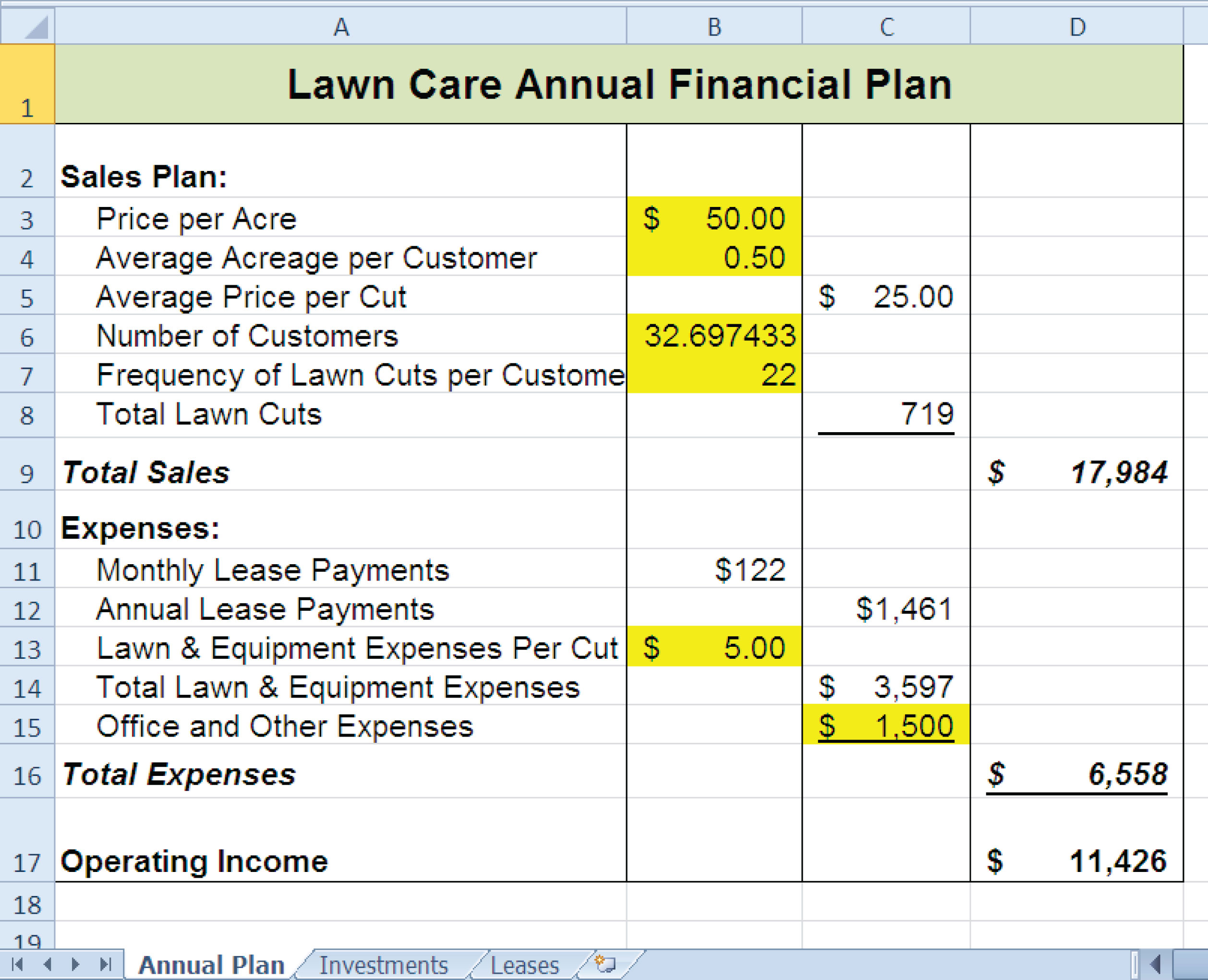
Figure 2.50 Completed CiP Exercise 1 Investments Worksheet
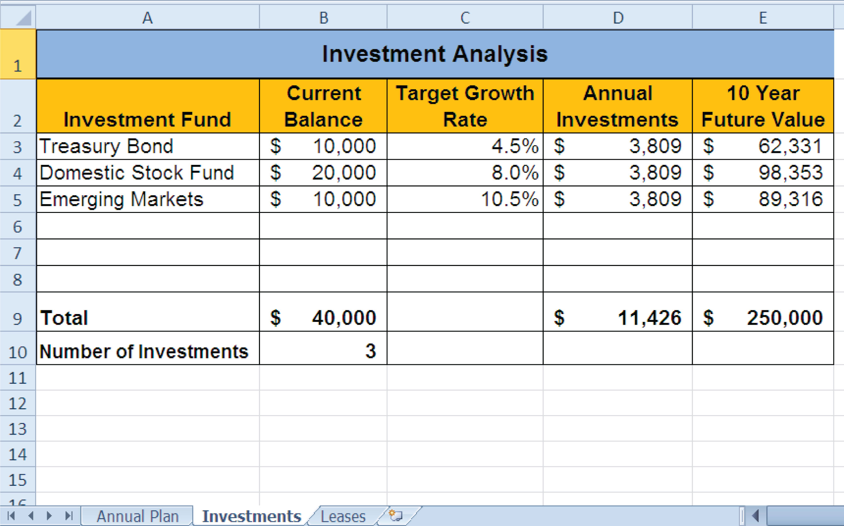
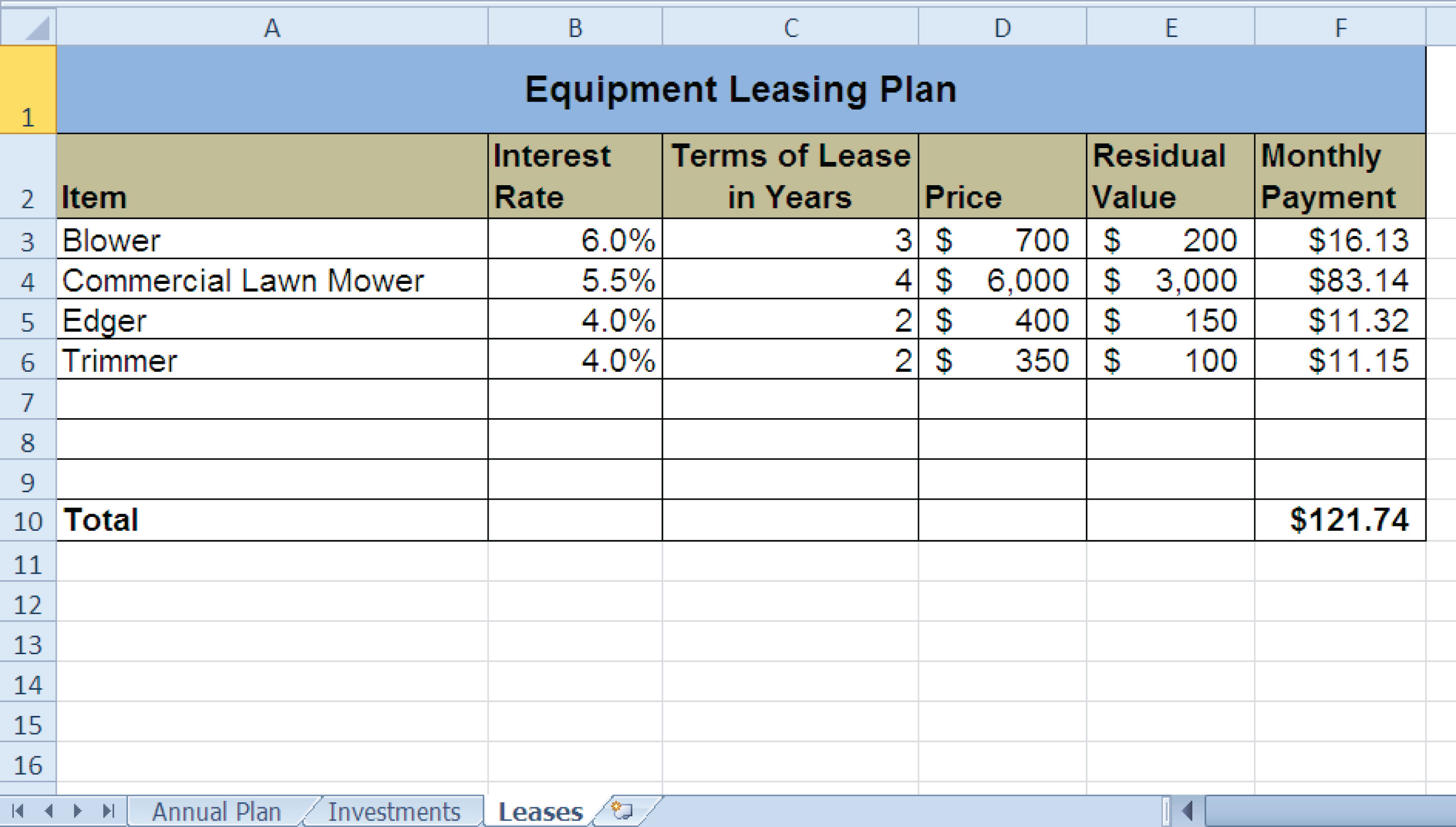
Figure 2.51 Completed CiP Exercise 1 Leases Worksheet
Hotel Management Cost Analysis
Starter File: Chapter 2 CiP Exercise 2
Difficulty: Level 2 Moderate
The hotel management industry presents a wide variety of career opportunities. These range from running your own bed and breakfast to a management position at a large hotel corporation. No matter what hotel management career you choose to pursue, understanding the costs for any hotel operation is critical to running a successful operation. This exercise examines the relationship between cleaning expenses and the occupancy rate of a small hotel. Cleaning expenses are obviously influenced by the occupancy rate of the hotel. As more rooms need to be cleaned, the amount of overall cleaning expenses increases. However, to accurately estimate these expenses, you need to know whether there is a baseline, or fixed portion, of these expenses that does not change no matter how many rooms need to be cleaned. In other words, if you pay a cleaning staff a fixed salary, it does not matter if they clean 1 room or 100 rooms; their salary will remain the same. However, you may need more cleaning supplies as the number of rooms that need to be cleaned increases. In addition, the replacement of guest necessities such as soap, shampoo, lotions, and so on will also increase as the number of rooms to be cleaned increases. This exercise will demonstrate how these costs can be estimated through a technique called the high-low method. Begin this exercise by opening the file named Chapter 2 CiP Exercise 2.
- Enter a formula in cell C5 on the Historical Costs worksheet to calculate the January capacity for the hotel. The capacity is calculated by multiplying the occupants per room (cell C3) by the number of rooms in the hotel (cell C2). This result is then multiplied by the number of days in the month (cell C5). Construct this formula so that relative referencing does not change cells C3 and C2 when the formula is pasted into other cell locations in Column C.
- Copy the formula in cell C5 and paste it into the range C6:C16. Use a paste method that does not remove the border at the bottom of cell C16.
- Enter a formula in cell E5 on the Historical Costs worksheet to calculate the occupancy capacity of the hotel. Your formula should divide the Hotel Capacity into the Actual Capacity. Format your result to a percentage with two decimal places. Then copy and paste the formula into the range E6:E16. Use a paste method that does not remove the border at the bottom of cell E16.
- Enter a function in cell C17 on the Historical Costs worksheet that sums the values in the range C5:C16. Copy the function and paste it into cells D17 and F17. Use a paste method that does not change the border on the right side of cell F17.
- Copy the formula in cell E16 and paste it into cell E17. Use a paste method that does not change the border at the bottom of cell E17.
- Sort the data in the Historical Costs worksheet based on the values in the Actual Occupancy column in descending order (largest to smallest). For any duplicate values in the Actual Occupancy column, sort using the values in the Cleaning Expenses column in descending order.
- On the Cost Analysis worksheet, enter a function into cell B3 that shows the highest value in the range D5:D16 in the Actual Occupancy column on the Historical Costs worksheet.
- On the Cost Analysis worksheet, enter a function into cell B4 that shows the lowest value in the range D5:D16 in the Actual Occupancy column on the Historical Costs worksheet.
- On the Cost Analysis worksheet, enter a function into cell C3 that shows the highest value in the range F5:F16 in the Actual Occupancy column on the Historical Costs worksheet.
- On the Cost Analysis worksheet, enter a function into cell C4 that shows the lowest value in the range F5:F16 in the Actual Occupancy column on the Historical Costs worksheet.
- On the Cost Analysis worksheet, format cells B3 and B4 with a comma and zero decimal places. Format cells C3 and C4 with US dollars with zero decimal places.
- On the Cost Analysis worksheet, enter a formula in cell B5 that subtracts the lowest actual occupancy value from the highest actual occupancy value. Copy this formula and paste it into cell C5.
- Enter a formula in cell C6 on the Cost Analysis worksheet that calculates that variable cost portion for the cleaning expenses per month. As mentioned in the introduction to this exercise, the cleaning expense contains costs that increase with each room that is cleaned. This is known as a variable expense and can be estimated by dividing the Actual Occupancy High Low Difference (cell B5) into the Cleaning Expenses High Low Difference (cell C5). Format the output of this formula to US dollars with two decimal places.
- Enter a formula in cell C7 on the Cost Analysis worksheet that calculates the fixed cost portion for the cleaning expenses per month. This is the amount of money that will be spent on cleaning expenses no matter how many rooms are cleaned. Since we have calculated the variable cost portion of the cleaning expense, we can now use it to calculate the fixed expense. To do this, subtract from the High Cleaning Expense (cell C3) the result of multiplying the variable expense (cell C6) by the High Actual Occupancy (cell B3). Format the result of the formula to US dollars with zero decimal places.
- Enter the number 3500 in cell C2 on the Cleaning Cost Estimates worksheet. Format the number with commas and zero decimal places.
- Apply a yellow fill color to cell C2 on the Cleaning Cost Estimates worksheet. This is being formatted to indicate to the user of this worksheet that a number is to be entered into the cell.
- On the Cleaning Cost Estimates worksheet, enter a formula in cell C3 that calculates the estimated cleaning expenses given the number that was entered into cell C2. Now that we have calculated the variable and fixed expenses on the Cost Analysis worksheet, we can use the results to estimate the cleaning expenses. The formula is a + bX, where a is the fixed cost, b is the variable cost, and X is the activity level that is typed into cell C2. The fixed cost is added to the result of multiplying the variable cost by the activity level in cell C2. Format the output of the formula to US dollars with zero decimal places.
- Save the workbook by adding your name in front of the current workbook name (i.e., “your name Chapter 2 CiP Exercise 2”).
- Close the workbook and Excel.
Figure 2.52 Completed CiP Exercise 2 Historical Costs Worksheet

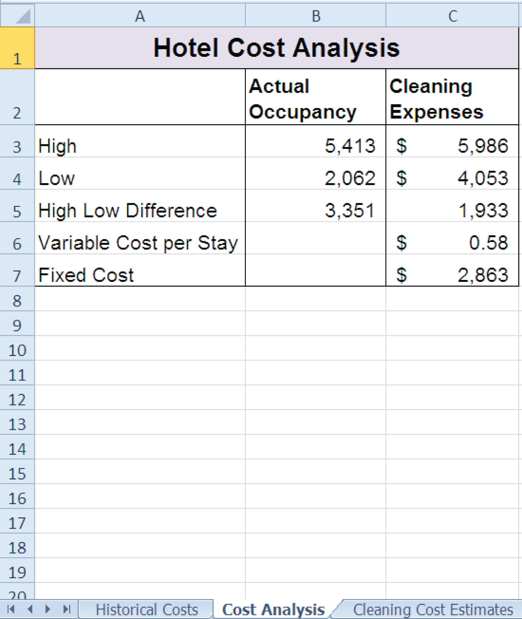
Figure 2.53 Completed CiP Exercise 2 Cost Analysis Worksheet
Integrity Check
Starter File: Chapter 2 IC Exercise 3
Difficulty: Level 3 Difficult
The purpose of this exercise is to analyze a worksheet to determine whether there are any integrity flaws. Read the scenario below, then open the Excel workbook related to this exercise. You will find a worksheet in the workbook named AnswerSheet. This worksheet is to be used for any written responses required for this exercise.
Scenario
You are the manager of a large do-it-yourself hardware store that is part of a national retail chain. Your assistant manager has constructed a sales and profit budget for the upcoming year. The Budget worksheet contains several formulas used to calculate the expected sales and profit dollars for the store by product category. The following is a list of key elements and calculations used on this worksheet:
- Cells shaded in yellow are intended for data entry values. For example, last year sales results in Column B are typed into the cells. Also, the expected growth rates in Column D and profit percentages in Column E are also typed into the cells. These values fluctuate from year to year, and the assistant manager intends to create a few scenarios for the budget by changing the growth rates and expected profit percentages for each product category.
- Table 2.9 "Formulas Used on the Budget Worksheet" contains a list of the formulas that are used to produce the outputs on the Budget worksheet.
Table 2.9 Formulas Used on the Budget Worksheet
| Purpose | Formula | Location |
|---|---|---|
| Budgeted Profit Dollars | Budgeted Sales × Profit Percent | F4:F7 |
| Budgeted Sales | Sales Last Year × (1 + Sales Growth) | C4:C7 |
| Total Profit Growth | (Total Budgeted Profit Dollars ÷ Total Budgeted Sales) | E8 |
| Total Sales Growth | (Total Budgeted Sales − Total Sales Last Year) ÷ Total Sales Last Year | D8 |
Assignment
- As noted in Table 2.9 "Formulas Used on the Budget Worksheet", the Sales Last Year is used in the formula calculating the Budgeted Sales dollars. Use the Trace Dependents command to locate the formula referencing any value in the Sales Last Year column on the Budget worksheet. Document your observation in the AnswerSheet worksheet.
- The assistant manager intends to use the Budget worksheet to create a few scenarios for the budgeted sales and profit dollars. Change a few values in the Profit Percent column and document your observations in the AnswerSheet worksheet.
- Look at each value in the Totals row (row 8) on the Budget worksheet. Are there any values that do not make sense? Type your answer on the AnswerSheet worksheet.
- Using Table 2.9 "Formulas Used on the Budget Worksheet" as a guide, evaluate all formulas that were entered into the Budget worksheet. Make any necessary corrections to the worksheet so when any value is changed in Columns B, D, and E, new outputs are created.
- Save the workbook by adding your name in front of the current workbook name.
Starter File: Chapter 2 IC Exercise 4
Difficulty: Level 3 Difficult
The purpose of this exercise is to analyze a worksheet to determine whether there are any integrity flaws. Read the scenario below, then open the Excel workbook related to this exercise. You will find a worksheet in the workbook named AnswerSheet. This worksheet is to be used for any written responses required for this exercise.
Scenario
Your friend is working on a few financial calculations in Excel and is asking for your assistance. The workbook that was given to you contains calculations for estimating the future value of investments and monthly mortgage calculations for purchasing a home. Your friend explained the following in an e-mail that was sent with the workbook:
- You will see in the Investment Plan worksheet that I have estimated the value of my investments in 5 years. My company is taking money out of my paycheck at the end of every month and investing it in the funds I have listed in Column A. I am pretty sure I did this right, but all my results in Column E are negative. I am not sure why this is happening.
- In the Mortgage Payments worksheet, I am trying to calculate the monthly payments for a house I am thinking about buying. However, the output of the function in cell B6 seems really high. There is no way I would be paying over $9,000 a month in mortgage payments. Something must be wrong.
- I don’t want to spend more than $775 a month for a mortgage. I thought I would be able to use Excel to determine what my target price for the house should be. My agent said that the current owners were probably willing to negotiate on the asking price for the house.
Assignment
- Look at the FV function that was entered into cell E3 on the Investment Plan worksheet. Why is the output for this function negative?
- Assume that the output of the FV function in cell E3 was a positive $17,385 instead of negative. Does it make sense that given a 4.5% annual rate of return, starting balance of $10,000, and an ongoing investment of $900 per month that the value of the investment would be $17,385 after 5 years?
- Look at the PMT function in cell B6 on the Mortgage Payments worksheet. Is the function set up to calculate monthly payments?
- You friend states that the target monthly mortgage payment is $775. What Excel tool could you use to change the price in cell B2 on the Mortgage Payments worksheet so the mortgage payment is equal to $775?
- Based on your friend’s comments, make any necessary corrections to all the functions in the Investment Plan and Mortgage Payments worksheets. Set the price of the home in cell B2 on the Mortgage Payments worksheet so the monthly payment equals $775.
- Save the workbook by adding your name in front of the current workbook name.
Applying Excel Skills
Lease vs. Buy
Starter File: None
Difficulty: Level 2 Moderate
You are in the process of getting a new car but are not sure if you should buy or lease. The price of the car you want is $18,000, but you do not want to spend more than $250 a month on car payments. If you lease the car, the terms of the lease will be 48 months at an annual interest rate of 5%. The residual value of the car will be set at $9,000. If you buy the car, your bank will offer you a 7-year loan at an annual interest rate of 6%. You are not required to make a down payment with either the lease or loan options, and payments are made at the end of the month for both options.
Should you lease or buy the car given your budget limit of $250 a month? Create a new workbook and design a worksheet that shows the difference between leasing and buying the car in terms of monthly payments. Use proper formatting so your worksheet is easy to read. Remember to use column and row headings, add a title to your worksheet, and rename the worksheet tab with an appropriate label. Include your name in the file name of the workbook.
Amortization Table for a Home Loan
Starter File: None
Difficulty: Level 3 Difficult
You are considering the purchase of a new home offered at a price of $225,000. Create an amortization table in a new workbook that shows how much interest and principal you will pay each month for the duration of the loan. The following is a list of assumptions and requirements you need to consider for this assignment:
- You will be making a down payment of 20% on the home (refer to Table 2.5 "Key Terms for Loans and Leases" for loan and lease terms).
- The bank will offer you a loan at an annual interest rate of 5.5% for 30 years.
- Your mortgage payments will be made at the end of each month.
- You must construct the amortization table so that any change in the loan variables, down payment percent, length of loan, interest rate, and so on will automatically produce new outputs for each month of the amortization table.
- The amortization table must show the interest payment, principal payment, and balance remaining to be paid on the loan for every month of the loan duration. The beginning balance for the last month of the loan should be equal to the principal payment in the last month. Refer to Figure 2.29 "Example of an Amortization Table" for establishing the format for the table.
- Remember to use column and/or row headings, add a title to your worksheet, and rename the worksheet tab with an appropriate label.
- Include your name in the file name of the workbook.
Chapter Skills Test
Starter File: Chapter 2 Skills Test
Difficulty: Level 2 Moderate
Answer the following questions by executing the skills on the starter file required for this test. Answer each question in the order in which it appears. If you do not know the answer, skip to the next question. Open the starter file listed above before you begin this test.
- Enter a function in cell B9 on the Investments worksheet that calculates the total of the values in the range B3:B8.
- Copy the function in cell B9 and paste it into cells C9 and G9.
- Enter a formula in cell E3 on the Investments worksheet that calculates the growth rate for the investments. Your formula should first subtract the value in the Invested Principal column from the value in the Current Balance column. Then, divide this result by the value in the Invested Principal column.
- Copy the formula in cell E3 and paste it into the range E4:E8.
- Copy the formula in cell E3 and paste it into cell E9 using the Paste Formulas option.
- Enter a formula in cell D3 on the Investments worksheet that divides the Current Balance by the total in cell C9. Add an absolute reference to C9 in this formula.
- Copy the formula in cell D3 and paste it into the range D4:D8.
- In cell G3 on the Investments worksheet, use the Future Value function to calculate the future value of the investment in 2 years. Use the Target Growth Rate to define the Rate argument. This is not an annuity so there are no periodic investments. Use the Current Balance to define the Pv argument. Assume that the investment is made at the beginning of the period.
- Copy the function in cell G3 and paste it into the range G4:G8.
- Enter a function in cell B10 on the Investments worksheet that calculates the average of the values in the range B3:B8.
- Copy the function in cell B10 and paste it into cells C10 and G10.
- On the Mortgage worksheet, use the data provided to enter a formula in cell B6 to calculate the principal of the loan that will be required to purchase the house.
- On the Mortgage worksheet, use the PMT function in cell B7 to calculate the monthly payments of the mortgage. Use cell locations from this worksheet to define each argument of the function. Assume that payments are made at the end of each month.
- On the Auto Lease worksheet, use the PMT function in cell B6 to calculate the monthly lease payments. Use cell locations from this worksheet to define each argument of the function. Assume that the lease payments are due at the beginning of each month.
- On the Auto Lease worksheet, use Goal Seek to change the Annual Interest rate in cell B2 so the monthly payments are exactly $200.
- In cell E2 on the Summary worksheet, use a cell reference to display the value in cell B9 in the Investments worksheet.
- In cell E3 on the Summary worksheet, use a cell reference to display the value in cell G9 in the Investments worksheet.
- Enter a formula in cell F4 on the Summary worksheet that subtracts the Principal of Investments from the 2 Year Future Value of Investments.
- Enter a formula in cell F5 on the Summary worksheet that calculates the amount of mortgage payments that will be made over 2 years. Your formula should multiply the value in B7 on the Mortgage worksheet by 24.
- Enter a formula in cell F6 on the Summary worksheet that calculates the amount of lease payments that will be made over 2 years. Your formula should multiply the value in B6 on the Auto Lease worksheet by 24.
- Enter a formula in cell F7 on the Summary worksheet that subtracts the sum of the values in the range F5:F6 from the value in cell F4.
- Sort the data in the range A2:G8 on the Investments worksheet. Sort the data based on the values in the Invested Principal column in ascending order (smallest to largest). For duplicate values in this column, sort using the values in the Target Growth Rate column in descending order (largest to smallest).
- Save the workbook by adding your name in front of the current workbook name (i.e., “your name Chapter 2 Skills Test”).
- Close the workbook and Excel.