This is “Logical Functions”, section 3.1 from the book Using Microsoft Excel (v. 1.0). For details on it (including licensing), click here.
For more information on the source of this book, or why it is available for free, please see the project's home page. You can browse or download additional books there. To download a .zip file containing this book to use offline, simply click here.


3.1 Logical Functions
Learning Objectives
- Learn how to use the Freeze Panes command to lock specific columns and rows in place while scrolling through large worksheets.
- Understand the construction and use of formulas, basic statistical functions, and financial functions.
- Learn how to construct a logical test to evaluate the contents of a cell location.
- Learn how to use the IF function to evaluate the data in a cell location using a logical test.
- Learn how to use the OR function within an IF function to evaluate the data in a cell location using multiple logical tests.
- Learn how to use the AND function within an IF function to evaluate the data in a cell location using multiple logical tests.
- Review the construction of nested IF functions for evaluating data using more than one logical test.
- Learn how to set a conditional format rule so formatting commands are automatically applied based on the value in a cell location.
This section reviews the use of logical functions in Excel through the construction of an investment portfolio. Although it may seem that managing investments is a specialized career choice, the reality is that almost everyone will become an investor at some point in their lives. Many companies offer employees retirement savings benefits through 401(k) or 403(b)Employee retirement savings plans offered by businesses and by public and private institutions. These plans allow you to deduct money from your paycheck every month, tax-free, and invest it. plans. These plans allow you to deduct money from your paycheck every month, tax-free, and invest it. In addition to the tax benefits afforded by such plans, many employers match a percentage of your monthly savings or deposit money into your retirement account as an added form of compensation. When you sign up for these savings plans, your company will give you a list of options as to how your money can be invested, and you choose the type of investments you would like the company to make on your behalf. As a result of this process, you become an investor. Excel can be an extremely valuable tool to help you make these investment decisions and analyze the performance of the money you have invested.
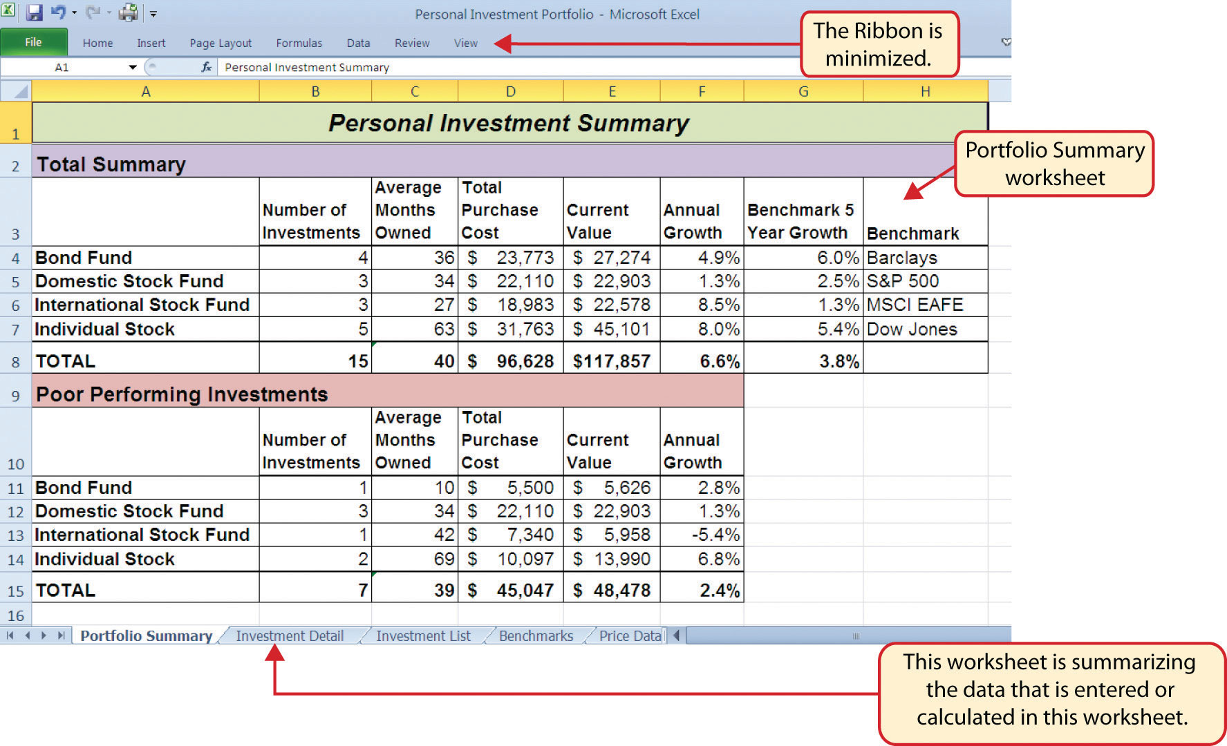
Figure 3.1 "Completed Personal Investment Portfolio Workbook" shows the completed investment portfolio workbook that we will complete in this chapter. Similar to the personal budget example in Chapter 2 "Mathematical Computations", the Portfolio Summary worksheet contains a summary of the data entered or calculated in other worksheets in the workbook. This project begins by building on the Investment Detail worksheet.
Figure 3.1 Completed Personal Investment Portfolio Workbook
Freeze Panes
Follow-along file: Excel Objective 3.00
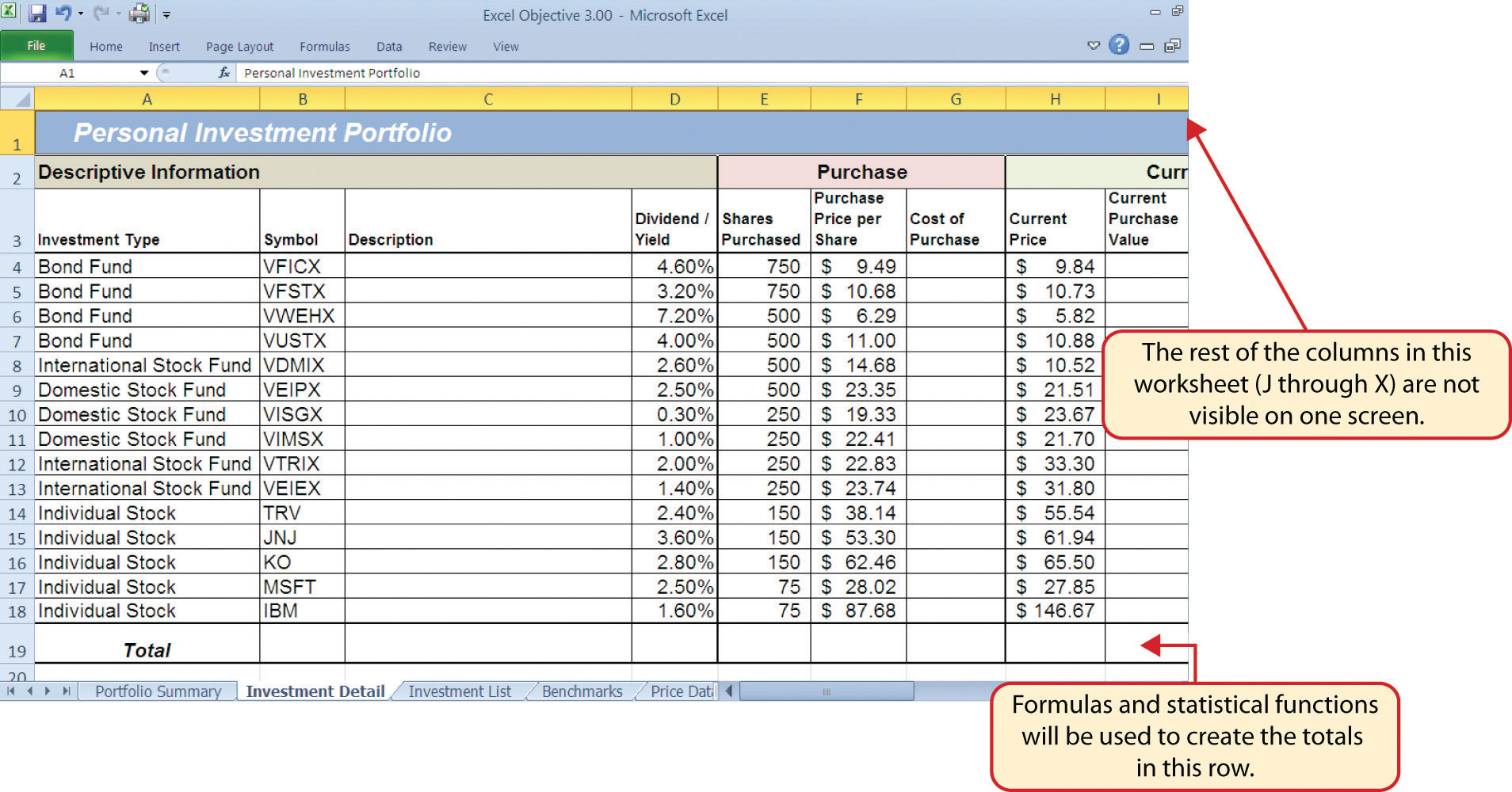
The Investment Detail worksheet shown in Figure 3.2 "Investment Detail Worksheet" contains the majority of the information used to create the Portfolio Summary worksheet shown in Figure 3.1 "Completed Personal Investment Portfolio Workbook". When you first open the worksheet, you will notice it is not possible to view all twenty-four columns on your computer screen. As you scroll to the right to view the rest of the columns, you will lose site of the row headings in Columns A and B. The headings in these columns show the investment that pertains to the data in Columns C through X. To solve this problem of viewing the row headings while scrolling through the remaining columns in the worksheet, we will use the Freeze Panes command.
Figure 3.2 Investment Detail Worksheet
The Freeze PanesAn Excel command that allows you to lock specific columns and rows in place while scrolling through a large worksheet. command allows you to scroll across the Investment Detail worksheet while keeping the row headings in Columns A and B locked in place. The following steps explain how to do this:
- Click cell C4 on the Investment Detail worksheet. We select this cell because the Freeze Panes option locks the columns to the left of the activated cell as well as the rows above the activated cell.
- Click the View tab on the Ribbon.
- Click the Freeze Panes button (see Figure 3.3 "Freeze Panes Command").
- Click the Freeze Panes option from the drop-down list of options.
Figure 3.3 Freeze Panes Command
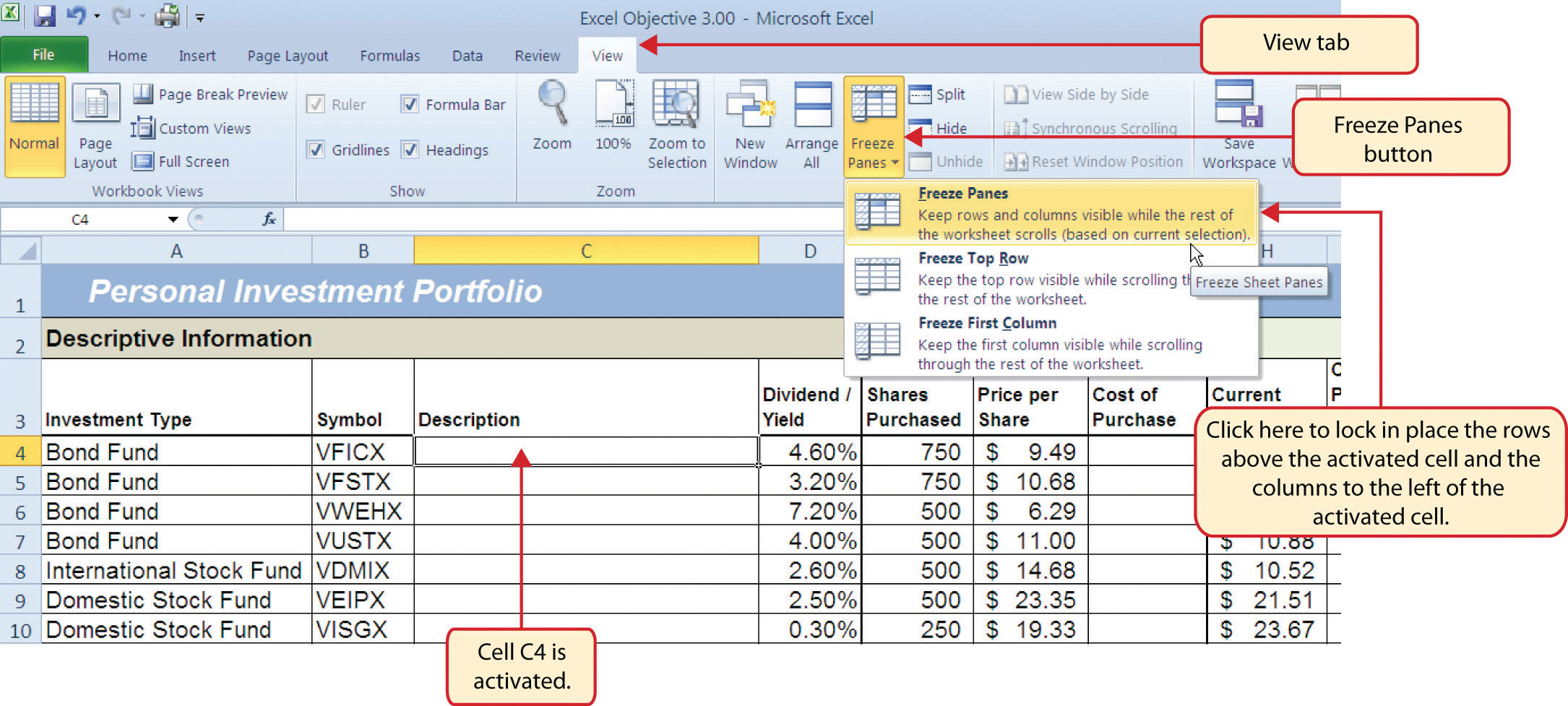
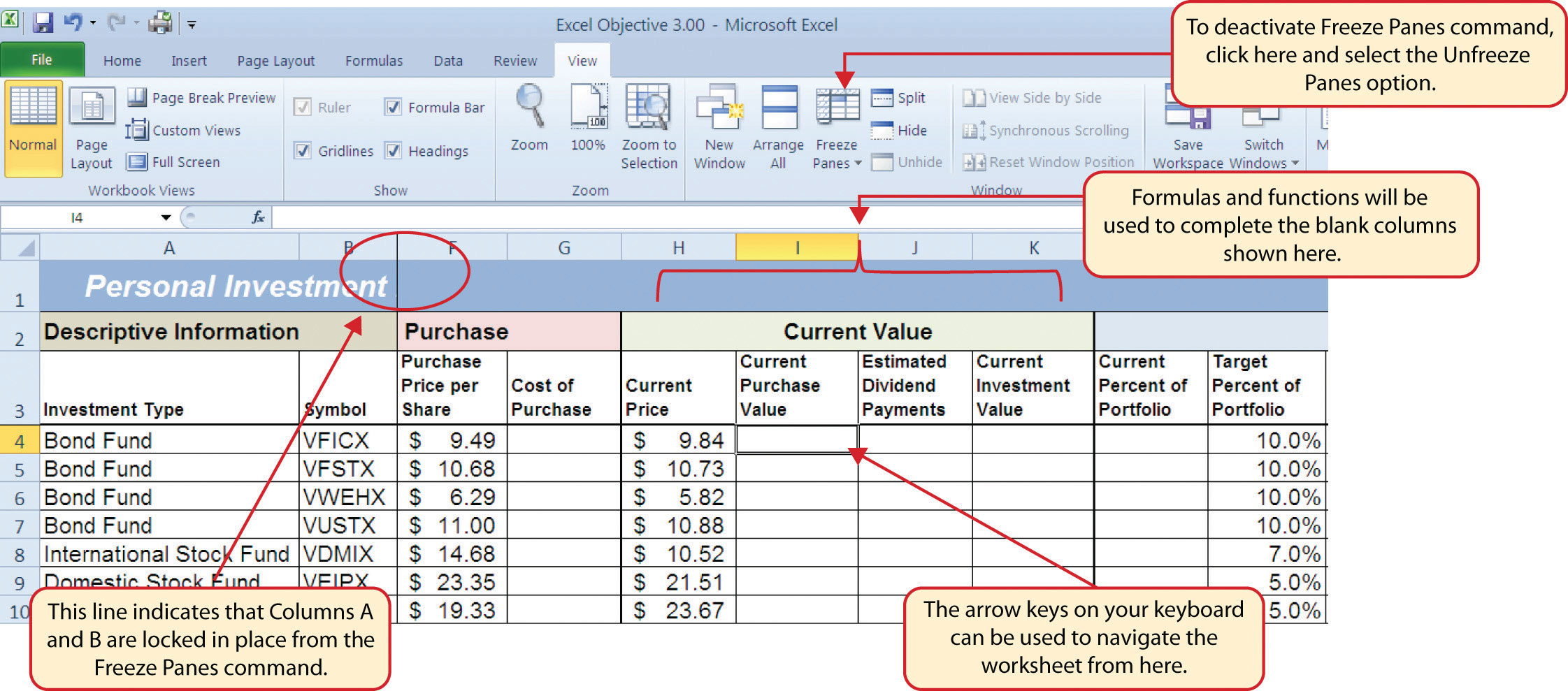
Once you click the Freeze Panes option shown in Figure 3.3 "Freeze Panes Command", Columns A and B are locked in place as you scroll through the columns in the worksheet. Since this is a large worksheet, you may find it easier to navigate the columns by using the arrow keys on your keyboard. However, since rows 1 and 2 contain merged cells, make sure a cell location is activated below Row 2 before you begin using the arrow keys. Figure 3.4 "Freeze Panes Command Activated on the Investment Detail Worksheet" shows the appearance of the Investment Detail worksheet after the Freeze Panes command has been activated. To deactivate the Freeze Panes command, click the Freeze Panes button again and select the Unfreeze Panes option.
Figure 3.4 Freeze Panes Command Activated on the Investment Detail Worksheet
Formula and Functions Review
Follow-along file: Continue with Excel Objective 3.00. (Use file Excel Objective 3.01 if starting here.)
We will begin developing the personal investment portfolio workbook by adding several formulas and functions. The formulas and functions we will add were illustrated in detail in Chapter 2 "Mathematical Computations". Therefore, the steps provided in this chapter will be brief. After the formulas and functions are added to the Investment Detail worksheet, we can add the logical and lookup functions. However, before proceeding, let’s review the investment type definitions in Table 3.1 "Investment Types in Column A of the Investment Detail Worksheet". Table 3.1 "Investment Types in Column A of the Investment Detail Worksheet" provides a definition for each of the investment types listed in Column A of the Investment Detail worksheet. This project assumes that the personal investment portfolio comprises four types of investments. The reason we include a variety of investment types in any portfolio is to manage our total risk, or potential of losing money. When building an investment portfolio, it is important to keep in mind that investments of all types can dramatically increase or decrease in value over a short period of time. Managing risk requires that your money is not concentrated in one type of investment.
Table 3.1 Investment Types in Column A of the Investment Detail Worksheet
| Category | Definition |
|---|---|
| Bond Fund | A mutual fund consisting of a variety of bonds. The benefit of buying shares of a fund as opposed to a specific bond is that doing so allows you to spread your investment over several bonds instead of concentrating your investment in just one bond. |
| Domestic Stock Fund | A mutual fund consisting of several domestic stocks. Buying shares of a stock mutual fund provides the benefit of investing your money over several stocks. |
| International Stock Fund | Same as a domestic stock fund but contains a variety of non-US or foreign stocks. |
| Individual Stock | The stock for one specific company. In addition to mutual funds, this chapter’s portfolio will include a few individual stocks for public companies. When you purchase shares of a specific company, such as IBM, you become a partial owner of that company. |
We will begin adding formulas and functions to the Investment Detail worksheet in sections. If you scroll across all the columns in the worksheet, you will notice the worksheet includes five distinct sections. Four of the five sections contain columns that need to be completed with formulas and functions before we can add the logical and lookup functions. Table 3.2 "Definitions for Columns A through G of the Investment Detail Worksheet" contains definitions for each of the columns in the Descriptive Information section (Columns A through D) and the Purchase section (Columns E through G). It will be helpful to understand the purpose of these columns as we complete this worksheet.
Table 3.2 Definitions for Columns A through G of the Investment Detail Worksheet
| Category | Definition |
|---|---|
| Investment Type | The type of investment with regard to bonds and stocks. A definition for each of the investment types used in this portfolio can be found in Table 3.1 "Investment Types in Column A of the Investment Detail Worksheet". |
| Symbol | The symbol that represents a mutual fund or stock. This symbol can be used to research the profile or current trading price on any website that provides stock quotes. |
| Description | The company name for an individual stock or a description of the type of investments made by a mutual fund. |
| Dividend/Yield | The amount of interest earned on a bond or bond fund or the amount of earnings distributed per share for an individual stock or stock fund. |
| Shares Purchased | The amount of shares purchased for a mutual fund or individual stock. |
| Purchase Price per Share | The price paid for the shares purchased for the mutual funds and individual stocks in the portfolio. |
| Cost of Purchase | The number of shares purchased multiplied by the purchase price per share. This represents your base investment and is used to determine how much money has been gained or lost. |
The Descriptive Information section of the Investment Detail worksheet (Columns A through D) contains only one blank column, which will be completed using a lookup function. Therefore, we will proceed to the Purchase section (Columns E through G) where the Cost of Purchase column is blank. The following steps explain how to enter the formula into this column:
- Click cell G4 on the Investment Detail worksheet.
- Type an equal sign (=).
- Enter a formula that multiplies the Shares Purchased (cell E4) by the Purchase Price per Share (cell F4).
- Copy the formula in cell G4.
- Highlight the range G5:G18.
- Click the down arrow on the Paste button in the Home tab of the Ribbon.
- Click the Formulas button from the list of options. This is the Paste Formulas command, which pastes only the formula without any associated formats for the copied cell location.
- Click cell E19 on the Investment Detail worksheet.
- Press and hold the ALT key on your keyboard, then press the equal sign (=). This is the shortcut for the Auto Sum feature.
- Press the ENTER key on your keyboard.
- Click cell G19 on the Investment Detail worksheet.
- Repeat step 9.
- Press the ENTER key on your keyboard.
Figure 3.5 "Completed Formula in the Cost of Purchase Column" shows the formula that was entered into cell G4 in the Purchase section of the Investment Detail worksheet. You can also see the results of the formula after it is pasted into the range G5:G18. The Paste Formulas option was used to paste the formula into this range so the borders would not be altered.
Figure 3.5 Completed Formula in the Cost of Purchase Column
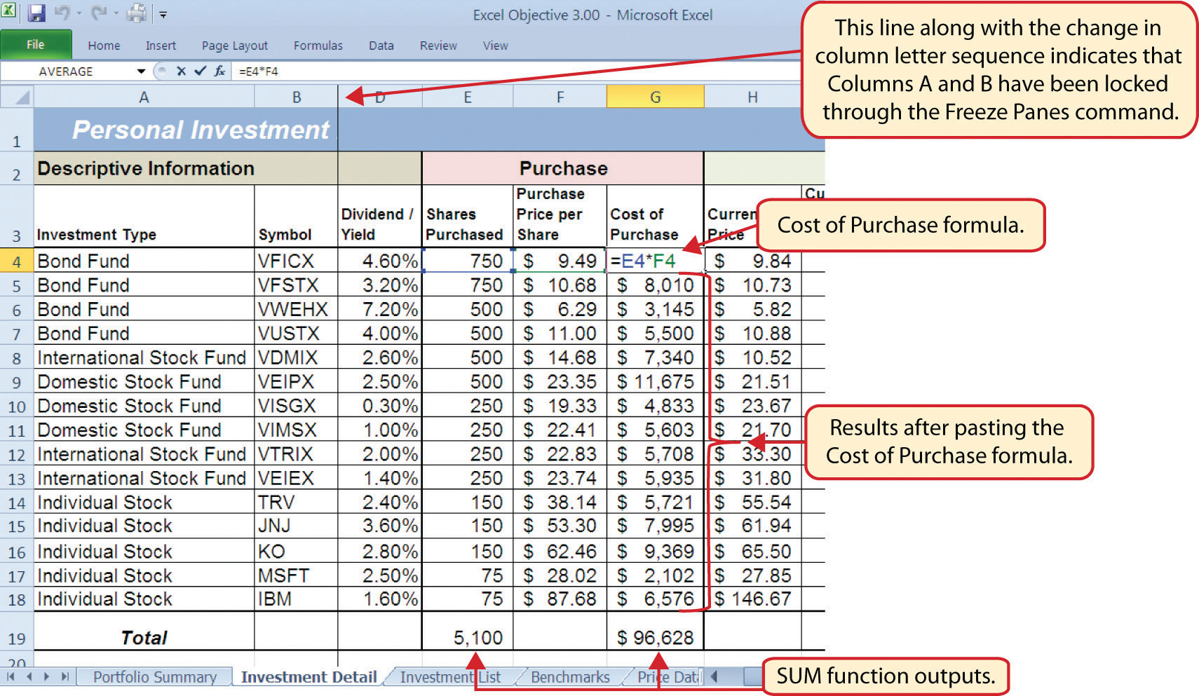
Table 3.3 "Definitions for Columns H through K of the Investment Detail Worksheet" shows the definitions for the Current Value section (Columns H through K) of the Investment Detail worksheet.
Table 3.3 Definitions for Columns H through K of the Investment Detail Worksheet
| Category | Definition |
|---|---|
| Current Price | The current price of an individual stock or the current net asset value of a mutual fund. |
| Current Purchase Value | The number of shares purchased multiplied by the current price. |
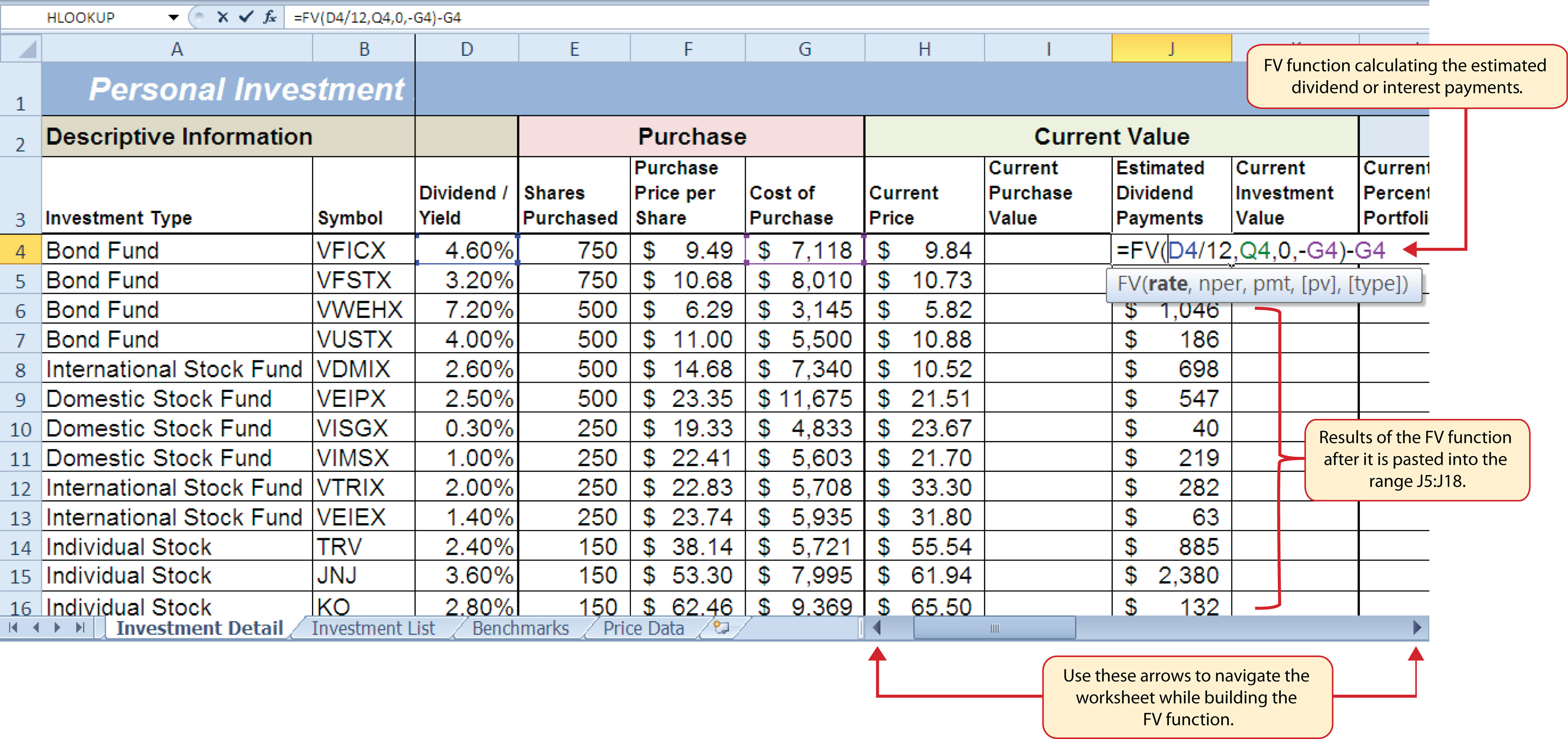
| Estimated Dividend Payments | The estimated amount of money paid for the interest on a bond fund or the dividends paid on a stock or stock fund. The future value function is used to estimate these payments. For an actual portfolio, real monetary distributions can be added to the current purchase value of the investment to calculate the total value of an investment. |
| Current Investment Value | The current purchase value plus the estimated dividend payments. The current investment value is compared with the cost of purchase to determine how much money is gained or lost. |
We will add a basic formula to the Current Purchase Value and Current Investment Value columns. For the Estimated Dividend Payments column, we will use the FV (future value) function to estimate the dividend payments. The following explains how we add the FV function to the Estimated Dividend Payments column:
- Click cell J4 and type an equal sign (=).
- Type the function name FV followed by an open parenthesis (().
- Click cell D4, type a forward slash (/) for division, and then type 12. This divides the rate in the Dividend/Yield column by 12. The length of ownership of an investment is expressed in terms of months in Column Q. Therefore, the rate for the FV function must be expressed in terms of months by dividing the annual rate by 12.
- Type a comma.
- Click cell Q4, which contains the number of months owned or the term of the future value calculation.
- Type a comma followed by a zero (,0). We are not calculating an annuity or periodic investment in this example, so the PMT argument will be defined with a zero. Type a comma to advance the function to the Pv argument.
- Type a minus sign (−) and click cell G4. This is the cost of the investment purchase previously calculated.
- Type a closing parenthesis ()).
- Type a minus sign (−) and click cell G4. By itself, the FV function is calculating the total value of the investment with dividends or interest earned. To show only the amount of dividends or interest earned, we subtract the cost of the investment purchase in G4 from the result of the FV function.
- Press the ENTER key on your keyboard.
- Adjust the decimal places for the output of the FV function to zero.
- Copy the FV function in cell J4 and paste it into the range J5:J18 using the Paste Formulas command.
Figure 3.6 "Completed FV Function in the Estimated Dividend Payments Column" shows the completed FV function in cell J4 of the Estimated Dividend Payments column. It is important to reduce the decimal places to zero after you enter the function into cell J4. Excel does not display the result of the function until the decimal places are removed because of the column width.
Figure 3.6 Completed FV Function in the Estimated Dividend Payments Column
The following steps explain how to add the formulas for the Current Purchase Value and Current Investment Value columns:
- Click cell I4 on the Investment Detail worksheet.
- Enter a formula that multiplies the Current Price in cell H4 by the Shares Purchased in cell E4.
- Copy the formula in cell I4 and paste it into the range I5:I18 using the Paste Formulas command.
- Click cell K4 on the Investment Detail worksheet.
- Enter a formula that adds the Current Purchase Value in cell I4 to the Estimated Dividend Payments in cell J4.
- Copy the formula in cell K4 and paste it into the range K5:K18 using the Paste Formulas command.
- Click cell K19 on the Investment Detail worksheet.
- Enter a SUM function that adds the values in the range K4:K18.
Figure 3.7 "Completed Current Value Section of the Investment Detail Worksheet" shows the completed columns of the Current Value section in the Investment Detail worksheet. The formula used to calculate the Current Investment Value illustrates why we used the FV function to calculate the estimated dividend or interest payments for an investment. Investments that earn interest or dividends can achieve growth in two ways. The first way is through interest or dividend payments. The second way is through changes in the price paid for the investment. The formula used to calculate the Current Purchase Value is taking the number of shares purchased for each investment and multiplying it by the current market price. Therefore, the Current Investment Value takes into account any changes in the investment price by adding the purchase value at the current market price to any dividends or interest payments earned.
Figure 3.7 Completed Current Value Section of the Investment Detail Worksheet
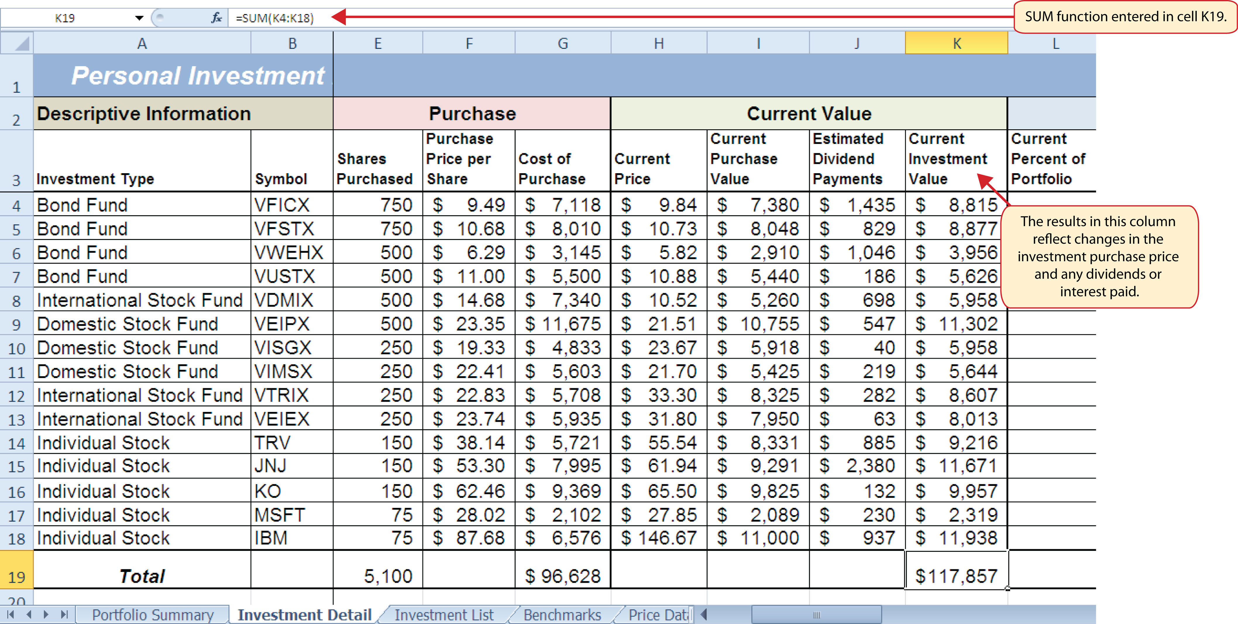
Table 3.4 "Definitions for Columns L through R of the Investment Detail Worksheet" provides definitions for the Percent of Portfolio section of the Investment Detail worksheet (Columns L through R).
Table 3.4 Definitions for Columns L through R of the Investment Detail Worksheet
| Category | Definition |
|---|---|
| Current Percent of Portfolio | The current investment value divided by the total current value of the investment portfolio. |
| Target Percent of Portfolio | The planned percentage each investment is intended to have for the entire portfolio. |
| Current vs. Target | The difference between the Current Percent of Portfolio column and the Target Percent of Portfolio column. |
| Rebalance Indicator | Shows which investments do not match the target percentage of the portfolio. For example, as one investment increases in value due to an increase in market price, it will comprise a greater percentage of the portfolio. This may require that some shares of this asset be sold and invested in other areas that may have decreased in value. This is known as rebalancing the portfolio, and it helps you sell investments when prices are high and buy investments when prices are low. |
| Buy/Sell Indicator | Based on the results of the Rebalance Indicator, a logical function is used to indicate whether an investment should be purchased or sold. |
| Months Owned | Shows how many months an investment is owned. The length of ownership is expressed in terms of months since dividend payments on stock funds and interest payments on bond funds are distributed monthly. |
| Long/Short Indicator | Shows whether an investment has been owned long enough to qualify as a long-term investment, which is greater than twelve months. The amount of taxes paid on the amount of money gained for a short-term investment is greater than a long-term investment. Therefore, there is a tax incentive to hold investments for more than twelve months. |
The Percent of Portfolio section of the Investment Detail worksheet (Columns L through R) requires two formulas and one function. The following steps explain how we add them to the worksheet:
- Click cell L4 in the Investment Detail worksheet.
- Enter a formula that divides the Current Investment Value in cell K4 by the total in cell K19.
- Place an absolute reference on cell K19 in the formula by placing the cursor in front of the column letter and pressing the F4 key on your keyboard.
- Copy the formula and paste it into the range L5:L18 using the Paste Formulas command.
- Click cell N4 in the Investment Detail worksheet.
- Enter a formula that subtracts the Target Percent of Portfolio (cell M4) from the Current Percent of Portfolio (cell L4): L4−M4.
- Copy the formula and paste it into the range N5:N18 using the Paste Formulas command.
- Click cell Q19 in the Investment Detail worksheet.
- Enter an AVERAGE function that calculates the average of the values in the range Q4:Q18.
Figure 3.8 "Percent of Portfolio Section of the Investment Detail Worksheet" shows the results of adding two formulas and a function to the Percent of Portfolio section of the Investment Detail worksheet. Notice the absolute reference added to the cell reference for K19 in the formula in the Current Percent of Portfolio column.
Figure 3.8 Percent of Portfolio Section of the Investment Detail Worksheet
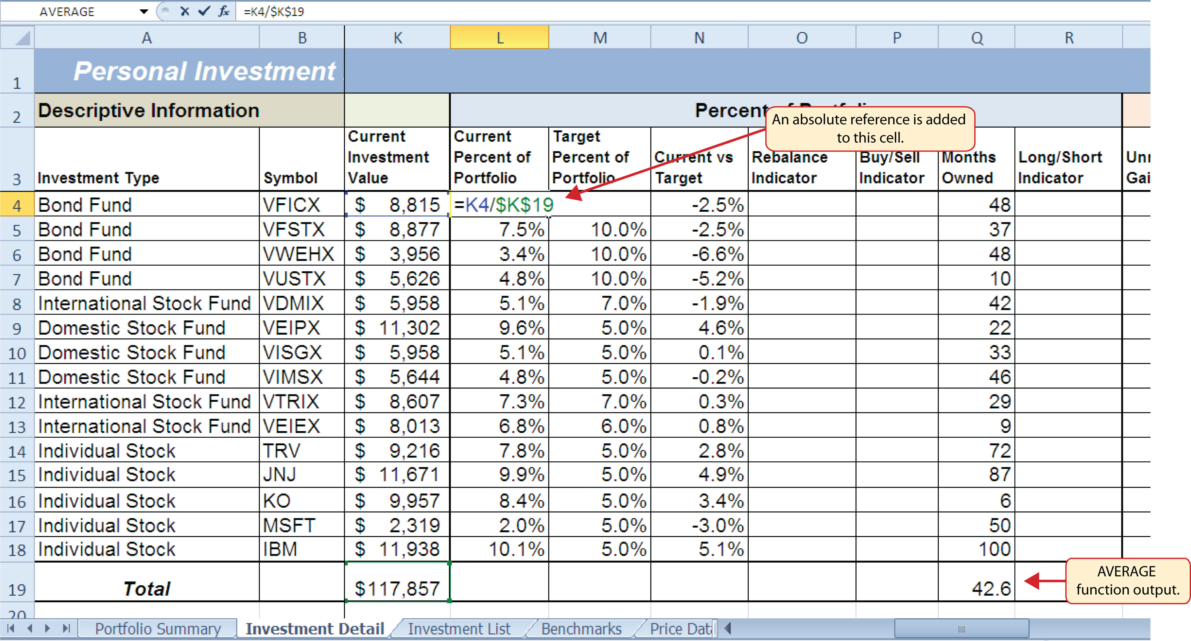
Table 3.5 "Definitions for Columns S through X of the Investment Detail Worksheet" provides definitions for the columns in the Performance Analysis section of the Investment Detail worksheet.
Table 3.5 Definitions for Columns S through X of the Investment Detail Worksheet
| Category | Definition |
|---|---|
| Unrealized Gain/Loss | The amount of money gained or lost on an investment. It is considered unrealized because the loss or gain does not actually occur until the investment is sold. |
| Percent Gain/Loss | The percentage increase or decrease based on the unrealized gain/loss and the purchase value of an investment. |
| Target Annual Growth Rate | The expected annual growth rate for an investment. All investments are expected to grow over time. The rate of growth depends on the amount of risk taken. Investments that are a higher risk are expected to pay a higher rate of return. |
| Actual Annual Growth Rate | The percentage gain/loss divided by the amount of time an investment is owned expressed in terms of years. |
| Target vs. Actual Growth Rate | The difference between the actual annual growth rate and the target annual growth rate. |
| Performance Indicator | A logical function will be used to indicate which investments are underperforming with respect to the target vs. actual growth rate. |
Most of the columns in the Performance Analysis section of the Investment Detail worksheet will be completed with formulas and functions. The following steps explain how we add them to the worksheet:
- Click cell S4 on the Investment Detail worksheet.
- Enter a formula that subtracts the value in the Cost of Purchase column (cell G4) from the value in the Current Investment Value column (cell K4): K4−G4.
- Copy the formula and paste it into the range S5:S19 using the Paste Formulas command. Note that this formula will be used to calculate the output for the Total row in this column. The results of the formula are showing how much money has been earned or lost for each investment. It is important to note that these gains or losses do not actually happen unless the investment is sold.
- Click cell T4 on the Investment Detail worksheet.
- Enter a formula that divides the Unrealized Gain/Loss (cell S4) by the Cost of Purchase (cell G4): S4/G4.
- Copy the formula in cell T4 and paste it into the range T5:T19 using the Paste Formulas command.
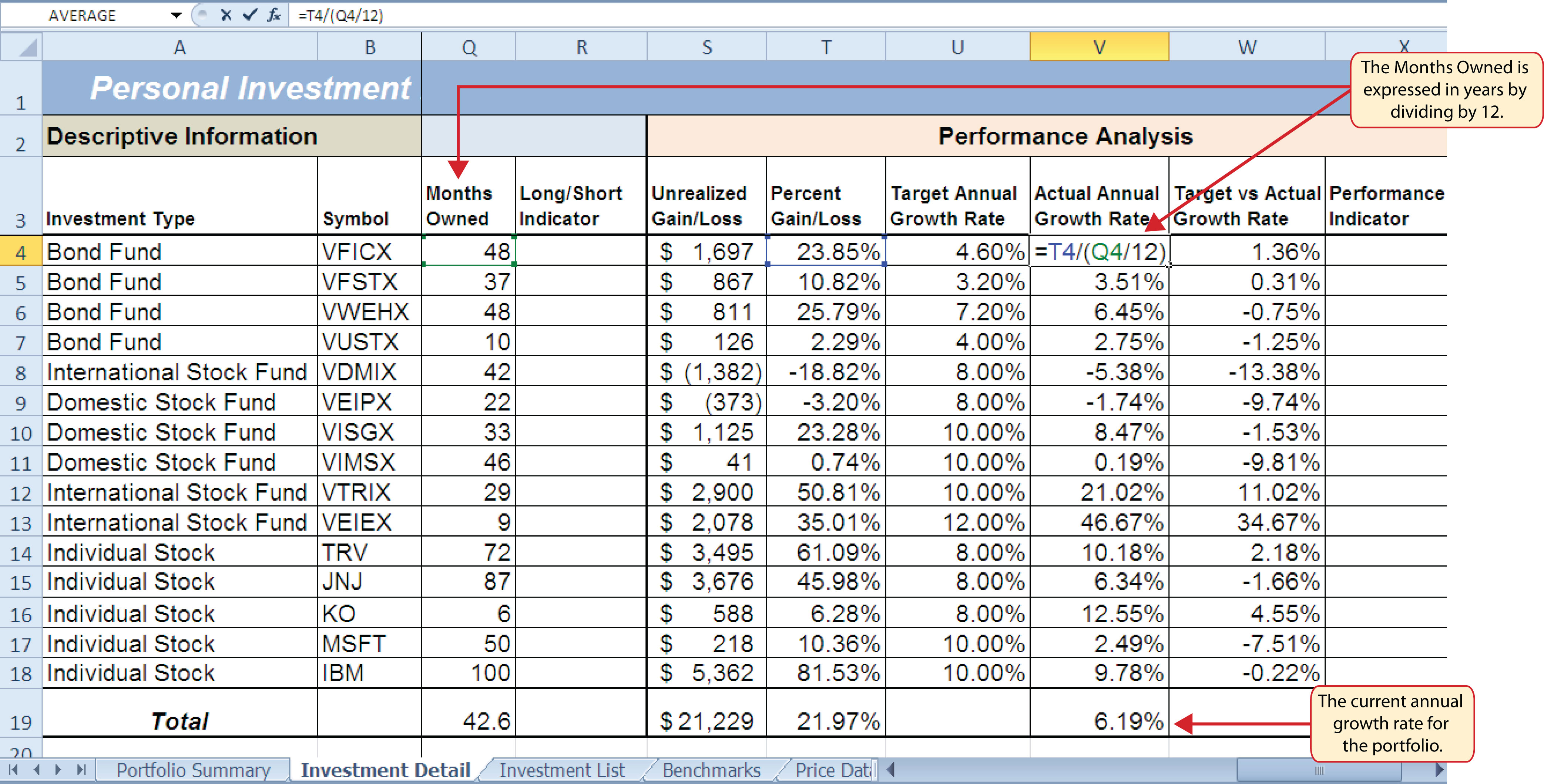
- Click cell V4 on the Investment Detail worksheet.
- Enter a formula that divides the Percent Gain/Loss (cell T4) by the result of dividing the Months Owned (cell Q4) by 12: T4/(Q4/12). Dividing the Months Owned value by 12 expresses the amount of time an investment has been owned in terms of years. The benchmark growth rates for most investments are expressed in terms of annual return rates. Therefore, this formula must first express the amount of time an investment has been owned in terms of years. Then the total percentage gain or loss for each investment is divided by the length of ownership in years to calculate the actual annual rate of return.
- Copy the formula in cell V4 and paste it into the range V5:V19 using the Paste Formulas command.
- Click cell W4 on the Investment Detail worksheet.
- Enter a formula that subtracts the Target Annual Growth Rate (cell U4) from the Actual Annual Growth Rate (cell V4): V4−U4.
- Copy the formula in cell W4 and paste it into the range W5:W18 using the Paste Formulas command.
Figure 3.9 "Performance Analysis Section of the Investment Detail Worksheet" shows the results of the formulas added to the Performance Analysis section of the Investment Detail worksheet. This completes the required formulas and functions necessary to add before moving on to the logical and lookup functions of the chapter.
Figure 3.9 Performance Analysis Section of the Investment Detail Worksheet
The Logical Test
Follow-along file: Continue with Excel Objective 3.00. (Use file Excel Objective 3.02 if starting here.)
A key component for the logical functions that will be demonstrated in this section is the logical testAn expression used to evaluate the contents of a cell location. The logical test typically contains comparison operators such as equal to (=), greater than (>), less than (<), and so on. The results of the logical test can be either true or false. An example of a logical test is B8 >= 25, which is read as “if the value in cell B8 is greater than or equal to 25.”. A logical test is used in logical functions to evaluate the contents of a cell location. The results of the logical test can be either true or false. For example, the logical test C7 = 25 (read as “if the value in cell C7 is equal to 25”) can be either true or false depending on the value that is entered into cell C7. A logical test can be constructed with a variety of comparison operators, as shown in Table 3.6 "Comparison Operator Symbols and Definitions". These comparison operators will be used in the logical test arguments for the logical functions demonstrated in this chapter.
Table 3.6 Comparison Operator Symbols and Definitions
| Symbol | Definition |
|---|---|
| = | Equal To |
| > | Greater Than |
| > | Less Than |
| < > | Not Equal To |
| > = | Greater Than or Equal To |
| < = | Less Than or Equal To |
A logical test will be used to evaluate the contents of a cell location in the Investment Detail worksheet. We will first demonstrate how the logical test is used to evaluate the contents of a cell location. Then we will use this logical test in the IF function, which will be demonstrated next. The following steps explain how the logical test is constructed:
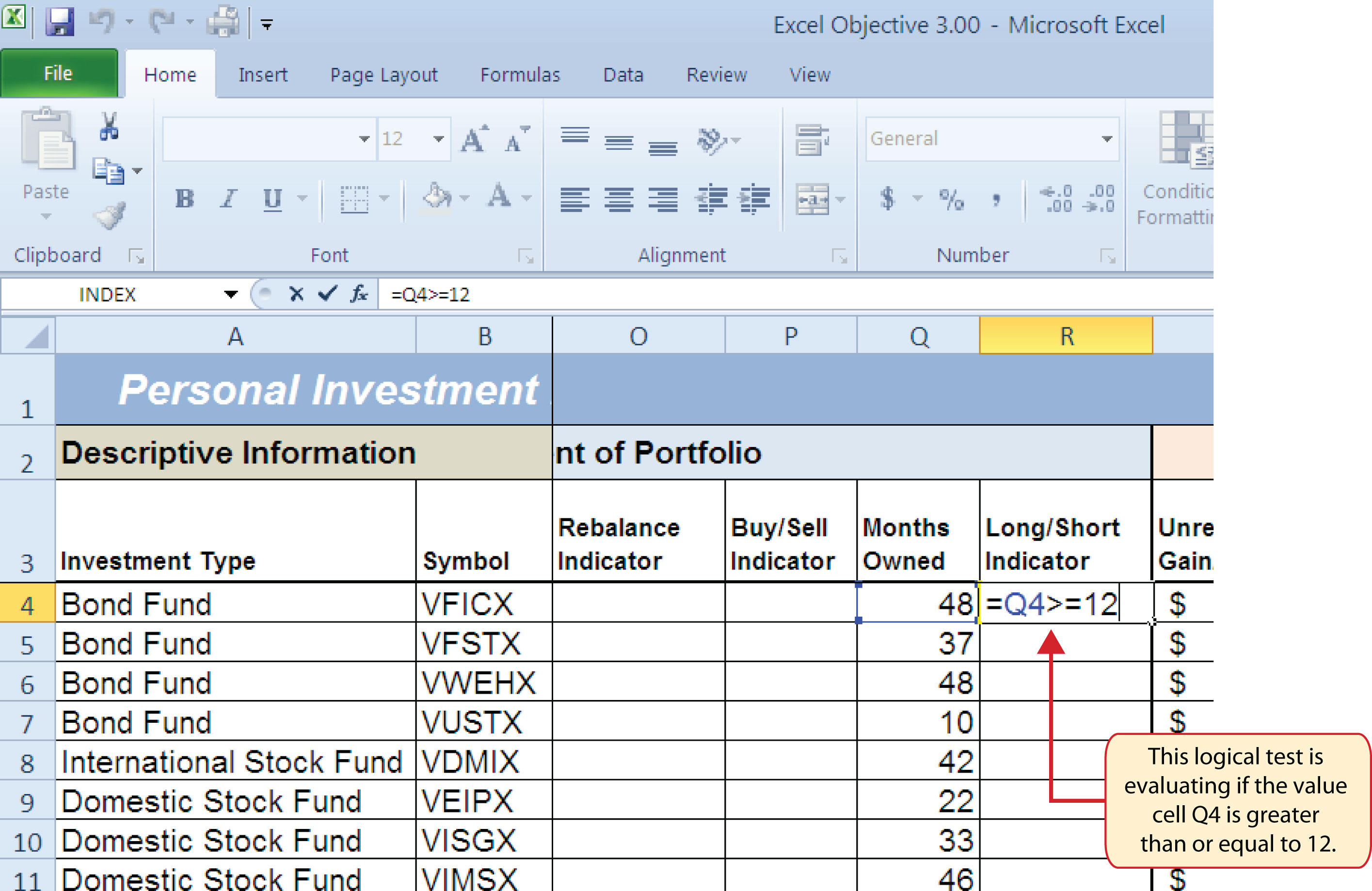
- Click cell R4 on the Investment Detail worksheet.
- Type an equal sign (=).
- Click cell Q4.
- Type the greater than sign (>) followed by an equal sign (=).
-
Type the number 12. This completes the logical test, which is shown in Figure 3.10 "Logical Test Entered into the Investment Detail Worksheet". The logical test would be stated as: “If the value in cell Q4 is greater than or equal to 12.”
Figure 3.10 Logical Test Entered into the Investment Detail Worksheet
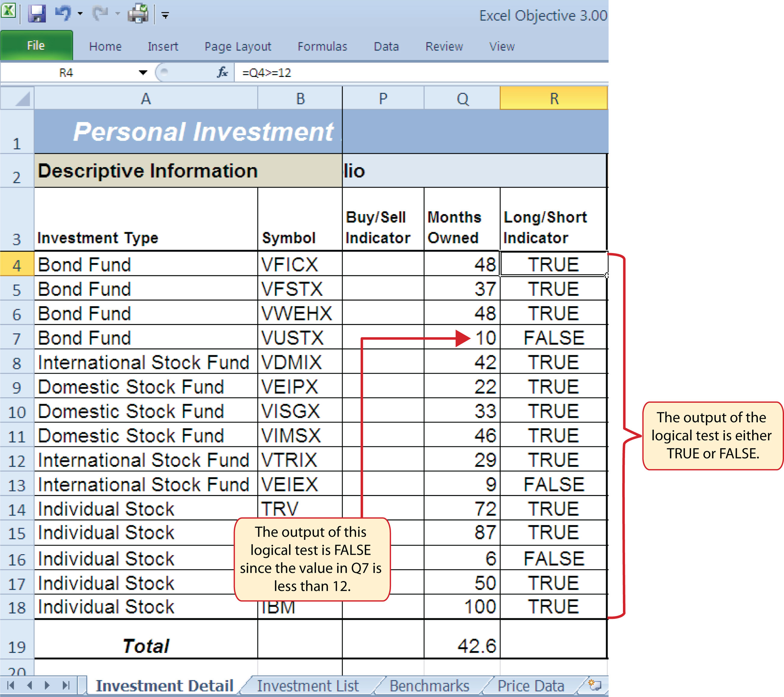
- Press the ENTER key on your keyboard. Notice that the output of the logical test is the word TRUE. This is because the value in cell Q4 is 48, which is greater than 12 (see Figure 3.11 "Output of the Logical Test").
- Copy the logical test in cell R4 and paste it into the range R5:R18 using the Paste Formulas command.
Figure 3.11 "Output of the Logical Test" shows the results of the logical test after it is pasted into the range R5:R18. Notice that for any values that are less than 12 in the range Q4:Q18, the logical test produces an output of FALSE.
Figure 3.11 Output of the Logical Test
IF Function
Follow-along file: Continue with Excel Objective 3.00. (Use file Excel Objective 3.03 if starting here.)
The IF function is used to produce a custom output based on the results of a logical test. If the results of the logical test are TRUE, the IF function can display a specific number or text, or perform a calculation. If the results of the logical test are FALSE, the IF function can display a different number or text, or perform a different calculation. The arguments of the IF function are defined in Table 3.7 "Arguments for the IF Function".
Table 3.7 Arguments for the IF Function
| Argument | Definition |
|---|---|
| Logical_test | A test used to evaluate the contents of a cell location. This argument typically utilizes comparison operators, which are defined in Table 3.6 "Comparison Operator Symbols and Definitions". The results of the test can be either true or false. For example, the test C7>25 would be read as if C7 is greater than 25. If the number 30 is entered into cell C7, the logical test is true. If you are evaluating a cell that contains text data, the text in the logical test must be placed inside quotation marks. For example, if you wanted to test if the word Long is in cell C7, the logical test would be C7 = “Long”. |
| [Value_if_true] | The output that will be displayed by the function or the calculation that will be performed by the function if the results of the logical test are true. This argument can be defined with a formula, function, number, or text. However, when defining this argument with a text output such as the word Long, it must be placed inside quotation marks (“Long”). |
| [Value_if_false] | The output that will be displayed by the function or the calculation that will be performed by the function if the results of the logical test are false. This argument can be defined with a formula, function, number, or text. However, when defining this argument with a text output such as the word Long, it must be placed inside quotation marks (“Long”). |
We will use the IF function in the Percent of Portfolio section of the Investment Detail worksheet. We will use the logical test that was previously demonstrated within the IF function to determine if an investment has been held for a short or long period of time. For tax purposes, an investment is considered short-term if it is held less than twelve months. This requires the investor to pay a higher tax percentage for any profit earned on the investment. An investment held twelve months or longer is considered a long-term investment. The following explains how the IF function is used to identify which investments are long term or short term:
- Highlight the range R4:R18 on the Investment Detail worksheet and press the DELETE key on your keyboard. This will remove the logical test and allow us to replace it with an IF function.
- Click cell R4 on the Investment Detail worksheet.
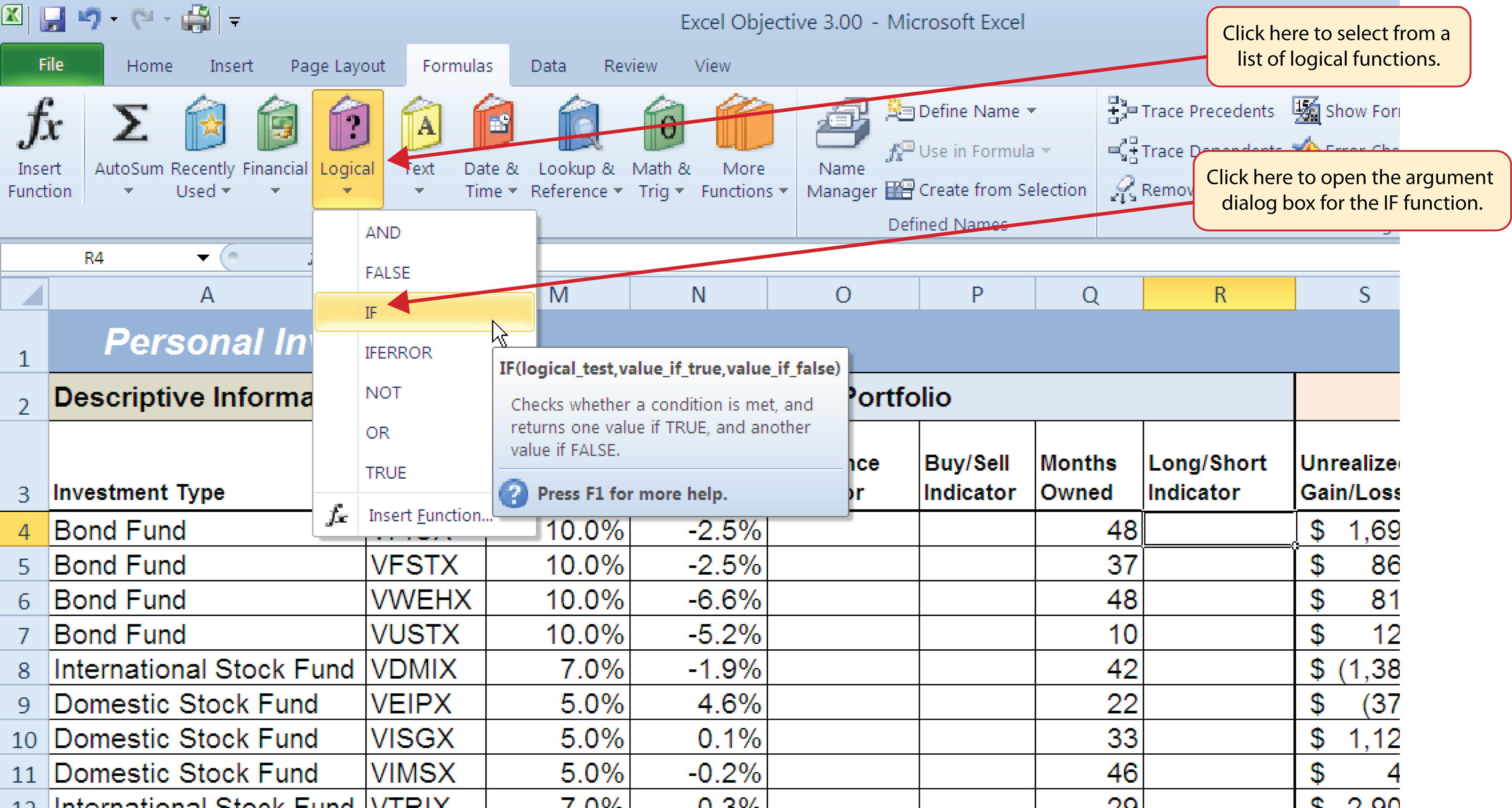
- Click the Formulas tab on the Ribbon.
- Click the Logical button in the Function Library group of commands.
-
Click the IF function from the list of functions (see Figure 3.12 "Selecting the IF Function from the Function Library"). This opens the Function Arguments dialog box.
Figure 3.12 Selecting the IF Function from the Function Library
- Click the Collapse Dialog button next to the Logical_test argument (see Figure 3.13 "Logical_Test Argument Defined").
- Click cell Q4 and press the ENTER key on your keyboard.
- Type the greater than sign (>) followed by an equal sign (=).
-
Type the number 12.
Figure 3.13 "Logical_Test Argument Defined" shows the appearance of the IF Function Arguments dialog box after defining the Logical_test argument. Notice that next to the Logical_test input box, Excel shows that the results of the test are true. This makes sense given that the value in cell Q4 is 48, which is greater than 12.
Figure 3.13 Logical_Test Argument Defined
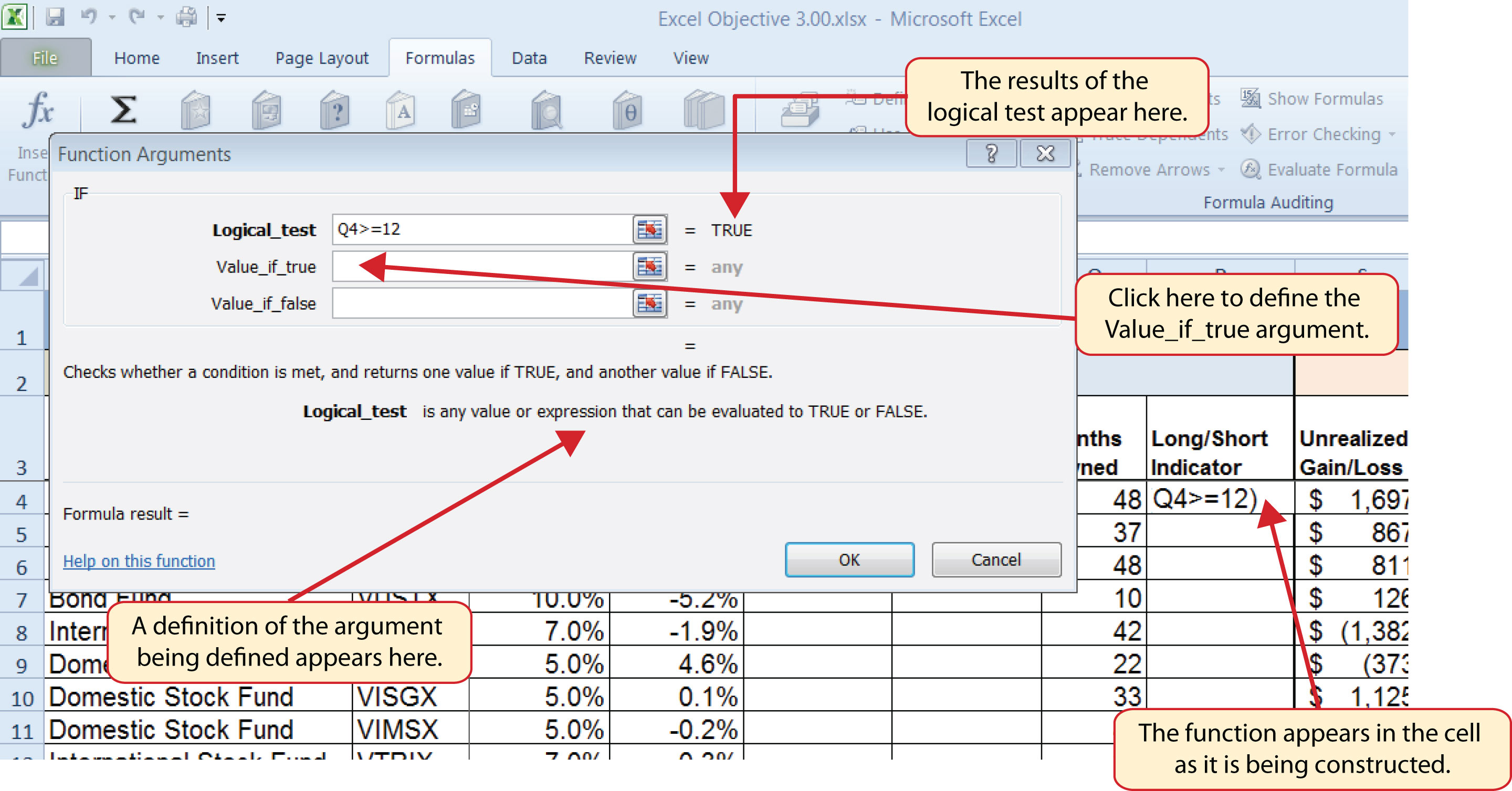
- Press the TAB key on your keyboard to advance to the next argument, which is Value_if_true.
- Type the word Long in quotation marks. If you forget to put words or text in quotation marks using the Function Arguments dialog box, Excel will insert the quotation marks for you.
- Press the TAB key on your keyboard to advance to the next argument, which is Value_if_false.
- Type the word Short in quotation marks.
- Click the OK button on the Function Arguments dialog box to complete the function.
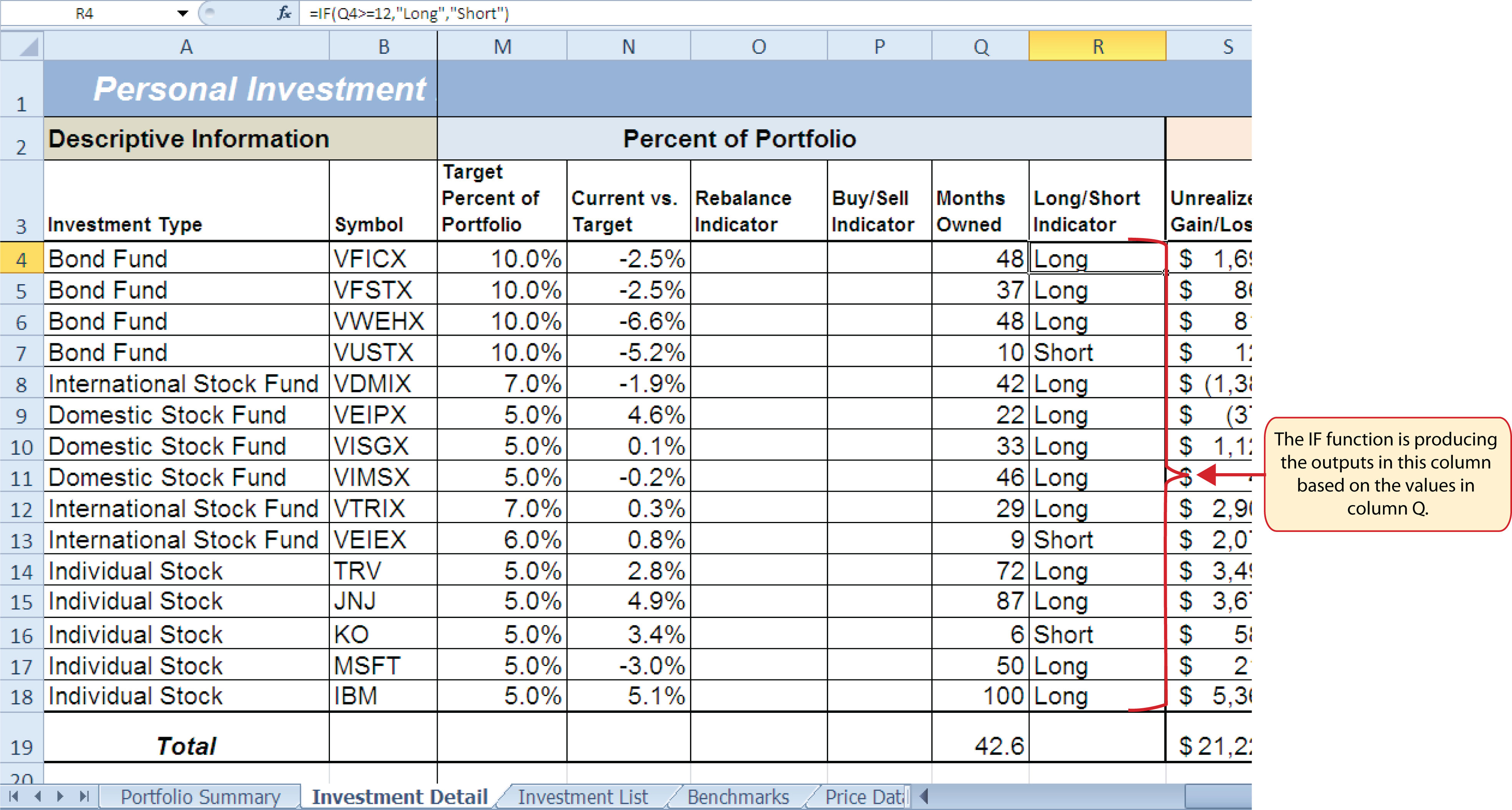
- Copy the IF function in cell R4 and paste it into the range R5:R18 using the Paste Formulas command.
Integrity Check
Placing Text in Quotation Marks for Logical Functions
If you are using a logical function to evaluate text data in a cell location, or if you are using a logical function to output text data, the text must be placed inside quotation marks. For example, if you are using a logical function to evaluate whether the word Long is entered into cell B5, the logical test must appear as follows: B5= “Long”. If you omit the quotation marks, the function may produce an erroneous false result for the test.
Figure 3.14 "Completed Function Arguments Dialog Box for the IF Function" shows the completed Function Arguments dialog box for the IF function. Notice that the results of the function are displayed in the dialog box. Since the value in cell Q4 is greater than 12, the word Long will be displayed in cell R4.
Figure 3.14 Completed Function Arguments Dialog Box for the IF Function
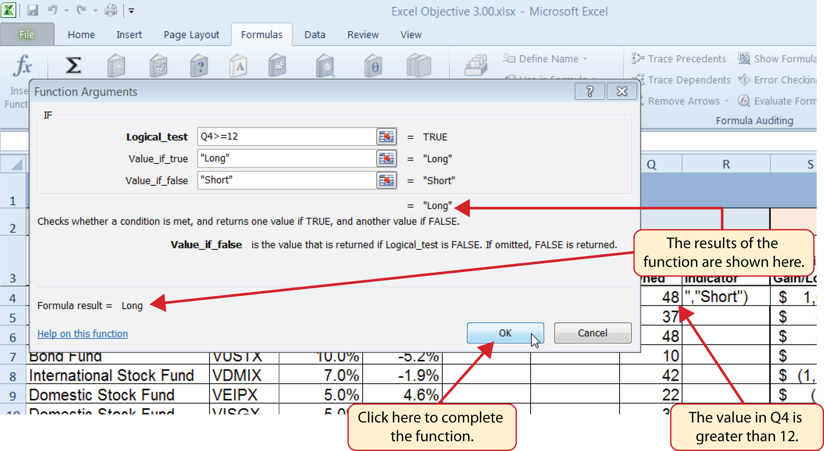
Figure 3.15 "IF Function Output" shows the completed Long/Short Indicator column on the Investment Detail worksheet. Notice the word Short is displayed for any investment held less than twelve months.
Figure 3.15 IF Function Output
Skill Refresher: IF and Nested IF Function
- Type an equal sign (=).
- Type the function name IF followed by an open parenthesis (().
- Define the logical_test argument to evaluate the contents of a cell location such that the result of the test is either true or false.
- Define the value_if_true argument, which will be the output of the function if the results of the logical test are true.
- Define the value_if_false argument, which will be the output of the function if the results of the logical test are false. This argument can also be defined by starting another IF function if you are nesting IF functions.
- Type a closing parenthesis ()). In the case of nested IF functions, type a closing parenthesis for every IF function that was started.
- Press the ENTER key on your keyboard.
The OR Function
Follow-along file: Continue with Excel Objective 3.00. (Use file Excel Objective 3.04 if starting here.)
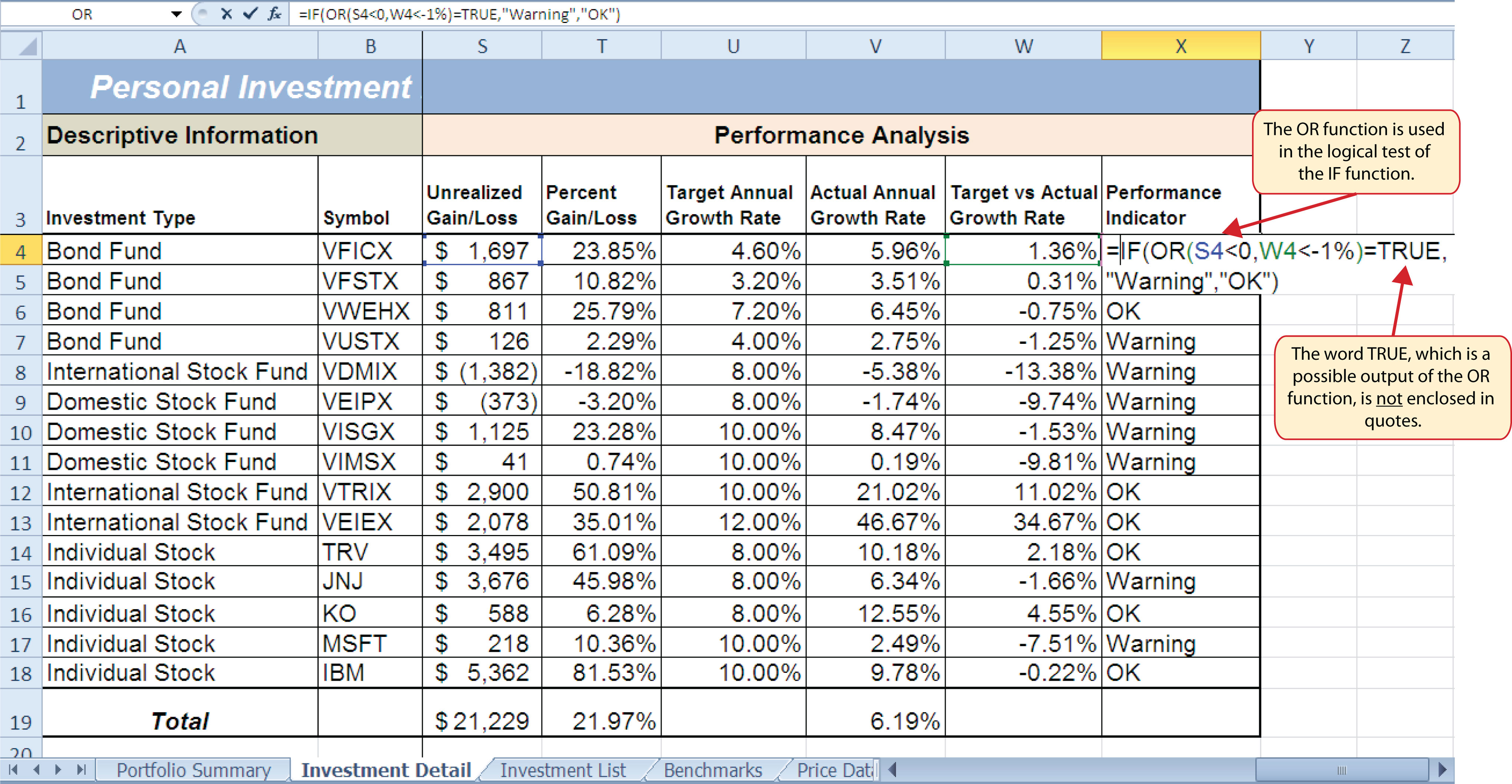
The OR function is similar to the IF function in that it uses a logical test to evaluate the contents of a cell location. However, the OR function allows you to define several logical tests as opposed to just one. If one of the logical tests is true, the output of the function will be the word TRUE. If all the logical tests are false, the output of the function will be the word FALSE. This differs from the IF function because the output of the function is only the word TRUE or the word FALSE. As a result, the OR function is commonly used within the IF function to enable specific outputs to be defined.
We will use the OR function in the Performance Indicator column on the Investment Detail worksheet. The purpose of this column is to identify any investment where either the Unrealized Gain/Loss is less than zero or the Target vs. Actual Growth Rate is less than –1%. We will use the function in the logical test of an IF function so we can define a specific output based on the results of the OR function. However, we will first demonstrate how the OR function works by itself, which is outlined in the following steps:
- Click cell X4 on the Investment Detail worksheet.
- Type an equal sign (=).
- Type the function name OR followed by an open parenthesis (().
- Click cell S4 on the Investment Detail worksheet.
- Type the less than symbol (<) followed by a zero. This completes the first logical test, which is evaluating if the value in cell S4 is less than zero.
- Type a comma. This advances the function to a second logical test.
- Click cell W4 on the Investment Detail worksheet.
- Type the less than symbol (<) followed by −1%. Be sure to include the minus sign and percent symbol. This completes the second logical test, which is evaluating if the value in cell W4 is less than –1%.
- Type a closing parenthesis ()) and press the ENTER key on your keyboard.
- Copy the OR function in cell X4 and paste it into the range X5:X18 using the Paste Formulas command.
Figure 3.16 Completed OR Function by Itself
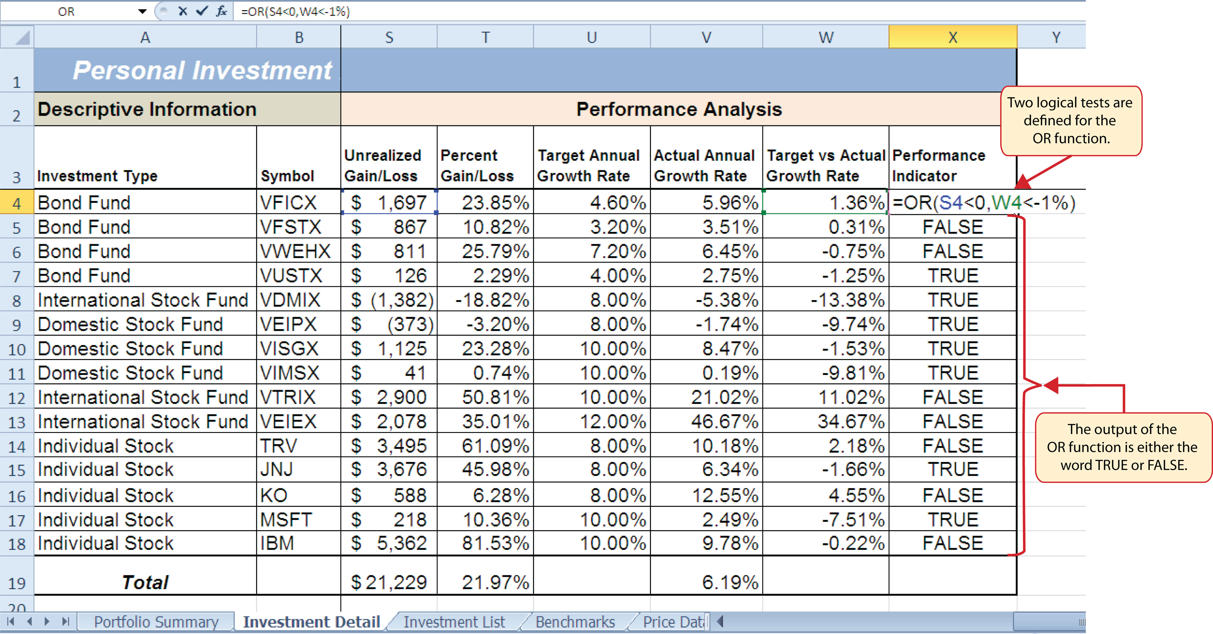
Figure 3.16 "Completed OR Function by Itself" shows the construction and result of the OR function by itself. Notice that the only output of the function is the word TRUE or the word FALSE. If either the Unrealized Gain/Loss is less than zero or the Target vs. Actual Growth Rate is less than −1%, the function shows the word TRUE. However, these descriptions will not be helpful for the person using this worksheet. Displaying the words OK or Warning would be far more helpful in identifying investments that need to be evaluated. We can do this if we use the OR function in the logical test argument of the IF function. The following steps explain how to accomplish this:
- Highlight the range X4:X18 on the Investment Detail worksheet and press the DELETE key on your keyboard. We are going to start over by creating an IF function.
- Click cell X4 on the Investment Detail worksheet.
- Type an equal sign (=).
- Type the function name IF followed by an open parenthesis (().
- Type the function name OR followed by an open parenthesis ((). The OR function is being placed into the logical_test argument of this IF function.
- Click cell S4 on the Investment Detail worksheet.
- Type the less than symbol (<) followed by a zero.
- Type a comma. This advances the function to a second logical test.
- Click cell W4 on the Investment Detail worksheet.
- Type the less than symbol (<) followed by −1%.
- Type a closing parenthesis ()).
- Type an equal sign (=).
- Type the word TRUE. Do not put the word inside quotation marks.
- Type a comma. This completes the logical_test argument of the IF function. We can now go on to define the value_if_true and the value_if_false arguments. This will allow us to specify what the output of the function should be instead, using the OR function outputs of either TRUE or FALSE.
- Type the word Warning. Be sure to enclose the word in quotation marks.
- Type a comma. This will advance the function to the value_if_false argument.
- Type the word OK. Be sure to enclose the word in quotation marks.
- Type a closing parenthesis ())and press the ENTER key on your keyboard.
- Copy the IF function in cell X4 and paste it into the range X5:X18 using the Paste Formulas command.
Figure 3.17 "OR Function in the Logical Test of the IF Function" shows the OR function within the logical_test argument of the IF function. The logical test of the IF function is now evaluating if the results of the OR function are true.
Figure 3.17 OR Function in the Logical Test of the IF Function
Skill Refresher: OR Function
- Type an equal sign (=).
- Type the function name OR followed by an open parenthesis (().
- Define the logical_test argument to evaluate the contents of a cell location such that the result of the test is either true or false.
- Define additional logical test arguments as needed. The output of the function will be TRUE if any of the logical tests are true.
- Type a closing parenthesis ()).
- Press the ENTER key on your keyboard.
The AND Function
Follow-along file: Continue with Excel Objective 3.00. (Use file Excel Objective 3.05 if starting here.)
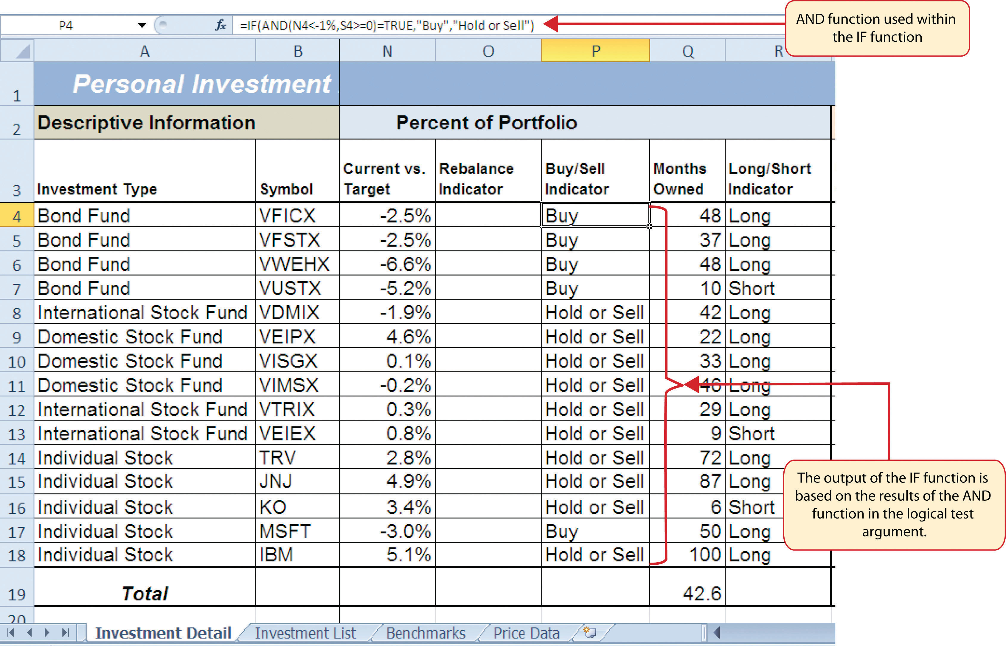
The AND function is almost identical to the OR function in that it is composed of only logical tests and produces one of two possible outputs: TRUE or FALSE. However, all logical tests defined for the AND function must be true in order to produce a TRUE output. If one logical test is false, the function will produce a FALSE output. We will use the AND function to complete the Buy/Sell Indicator column on the Investment Detail worksheet. This column will show either the word Buy or the words Hold or Sell based on the results of the logical test argument of an IF function. We will use the AND function to define the logical test argument of the IF function. The following steps explain how to accomplish this:
- Click cell P4 on the Investment Detail worksheet.
- Type an equal sign (=).
- Type the function name IF followed by an open parenthesis (().
- Type the function name AND followed by an open parenthesis ((). The AND function is being placed into the logical_test argument of this IF function.
- Click cell N4 and then type the less than symbol (<</b>).
- Type a minus sign (−) followed by the number 1 and a percent symbol: (−1%).
- Type a comma. This advances the AND function to the second logical test.
- Click cell S4.
- Type a greater than symbol (>) followed by an equal sign (=). These symbols are used to evaluate if the value in a cell location is greater than or equal to a target value.
- Type a zero followed by a closing parenthesis ()).
-
Type an equal sign (=) followed by the word TRUE. Do not enclose the word in quotation marks.
Figure 3.18 "AND Function Placed in the Logical Test of an IF Function" shows the appearance of the AND function that has been added to the logical test of the IF function. The AND function will produce a true output if the value in cell N4 is <−1% and the value in cell S4 is greater than or equal to 0.
Figure 3.18 AND Function Placed in the Logical Test of an IF Function
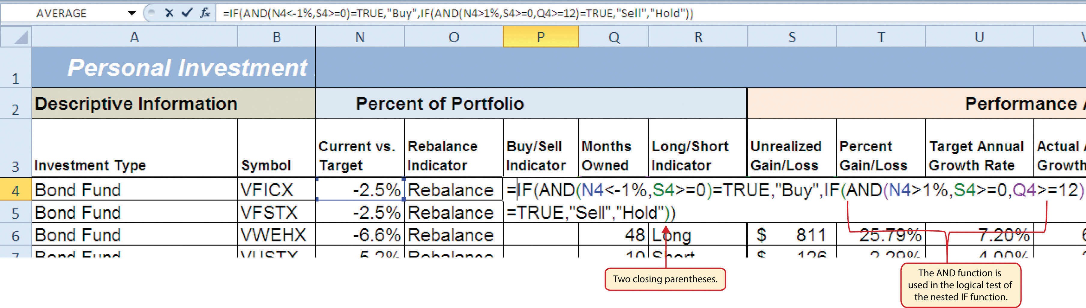
- Type a comma. This advances the IF function to the value_if_true argument.
- Type the word Buy enclosed in quotation marks as shown in Figure 3.19 "Results of the AND Function in the Logical Test Argument of an IF Function". If the Current vs. Target value is less than −1% and the Unrealized Gain/Loss is greater than or equal to zero, the function will show the word Buy. In other words, if the investment is less than the desired percentage for the total portfolio and it is currently not losing money, we will buy more of that investment so it is in line with the target percentage of the portfolio.
- Type a comma.
- Type the words Hold or Sell enclosed in quotation marks as shown in Figure 3.19 "Results of the AND Function in the Logical Test Argument of an IF Function". For all other investments that are not designated with a Buy indicator, the function will show the words Hold or Sell. This indicates that an investment could either be held or sold.
- Type a closing parenthesis ()) and press the ENTER key on your keyboard.
- Copy the IF function in cell P4 and paste it into the range P5:P18 using the Paste Formulas command.
- Increase the width of Column P to 12 points.
Figure 3.19 "Results of the AND Function in the Logical Test Argument of an IF Function" shows the results of the completed AND function within an IF function after it is copied and pasted into the range P5:P18.
Figure 3.19 Results of the AND Function in the Logical Test Argument of an IF Function
Skill Refresher: AND Function
- Type an equal sign (=).
- Type the function name AND followed by an open parenthesis (().
- Define the logical_test argument to evaluate the contents of a cell location such that the result of the test is either true or false.
- Define additional logical test arguments as needed. The output of the function will be TRUE if ALL of the logical tests are true.
- Type a closing parenthesis ()).
- Press the ENTER key on your keyboard.
Nested IF Functions
Follow-along file: Continue with Excel Objective 3.00. (Use file Excel Objective 3.06 if starting here.)
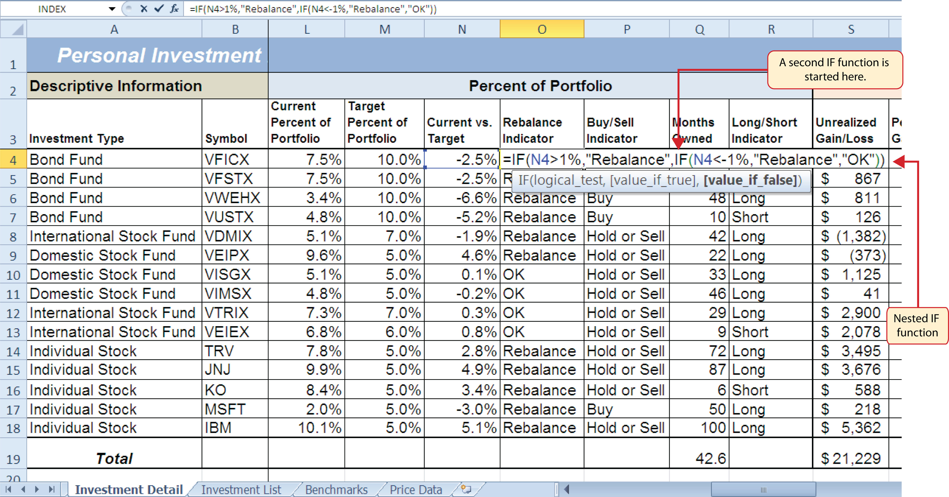
When constructing the IF function, the logical test can produce only two potential outcomes when evaluating the data in a cell. In addition, the function can produce only two possible outputs, which are defined in the value_if_true and value_if_false arguments. However, there may be situations when you need to test for several possible outcomes, which may require more than two possible outputs. To accomplish this, you need to create a nested IF functionUsed when more than two tests and two outputs are required when using the IF function. A nested IF function is when the value_if_true or value_if_false arguments of an IF function are defined with another IF function.. A nested IF function is when either the value_if_true or value_if_false arguments are defined with another IF function.
For the Personal Investment workbook, a nested IF function is required to complete the Rebalance Indicator column (Column O) on the Investment Detail worksheet (see Figure 3.19 "Results of the AND Function in the Logical Test Argument of an IF Function"). The purpose of this column is to indicate where the portfolio needs to be rebalanced. Looking at the Current vs. Target column (Column N) shown in Figure 3.19 "Results of the AND Function in the Logical Test Argument of an IF Function", you can see that several investments have a significant negative number where the investment value has fallen below the target percentage for the portfolio. Other investments have a significant positive number where the investment has exceeded the target percentage for the portfolio. For this portfolio, a number greater than 1% or less than –1% will be considered significant. Therefore, we will need to assess three possible outcomes when creating a logical test that evaluates the values in Column N. The first test will be if the value is greater than 1%. The second test will be if the value is less than –1%. The third test will be if both the first test and the second test are false. This is why we need to construct a nested IF function to produce the outputs in the Rebalance Indicator column. The following steps explain how to accomplish this:
- Click cell O4 on the Investment Detail worksheet.
- Type an equal sign (=).
- Type the function name IF followed by an open parenthesis (().
- Click cell N4.
- Type the greater than symbol (>) followed by the number 1%. It is important to use the percent symbol (%) after the number 1. If you omit the percent symbol, Excel will test if the value in cell N4 is greater than 100%.
- Type a comma.
- Type the word Rebalance inside quotation marks. When using text data to define any of the arguments for the IF function, the text must be placed inside quotation marks.
- Type a comma.
- Start another IF function by typing the function name IF followed by an open parenthesis (().
- Click cell N4.
- Type the less than symbol (<) followed by −1%.
- Type a comma.
- Type the word Rebalance inside quotation marks.
- Type a comma.
- Type the word OK inside quotation marks.
- Type two closing parentheses ())). Since two IF functions were started, there are two open parentheses in the function. As a result, we need to add two closing parentheses; otherwise, Excel will produce an error message stating that a closing parenthesis is missing.
- Press the ENTER key on your keyboard.
- Copy the nested IF function in cell O4 and paste it into the range O5:O18 using the Paste Formulas command.
Integrity Check
Using Logical Functions to Evaluate Percentages
If you are using a logical function to evaluate percentages in a cell location, be sure to use the percent symbol when defining the logical test. For example, if you are testing cell location B5 to determine if the value is greater than 10%, the logical test should appear as follows: B5>10%. If you omit the percent sign, the logical test will evaluate cell B5 to see if the value is greater than 1000%. This may erroneously force the function to produce the value_if_false output. You can also convert the percentage to a decimal in the logical test. For example, in decimal form, the logical test can be constructed as follows: B5>.10.
Figure 3.20 "Completed Nested IF Function" shows how the completed nested IF function should appear in cell O4 of the Investment Detail worksheet. In addition, we see the results of the function after it was pasted into the range O5:O18. Notice that for any investment where the Current vs. Target value is between plus or minus 1%, the word OK appears.
Figure 3.20 Completed Nested IF Function
Why?
Use AND or OR functions within IF functions
The benefit of using the AND or OR functions within the IF function is that doing so reduces the need to construct lengthy nested IF functions. It becomes increasingly difficult to manage the accuracy of lengthy nested IF functions. The AND and OR functions allow you to test for a variety of conditions in a cell location, which can reduce the need to nest multiple IF functions. Examine the nested if function in cell O4 on the Investment Detail worksheet. Can you recreate this without nesting the IF function?
Basic Conditional Formats
Follow-along file: Continue with Excel Objective 3.00. (Use file Excel Objective 3.07 if starting here.)
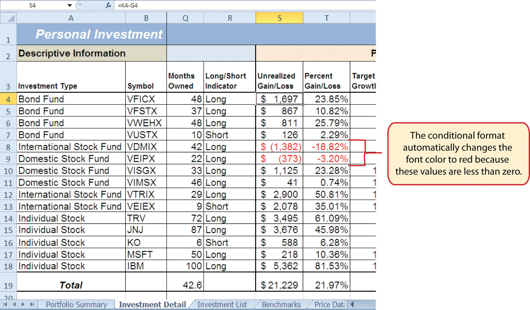
A feature related to the skills used to create logical functions is conditional formatting. Conditional formatsAn Excel feature that applies formatting commands to cell locations based on the cell contents. A basic conditional formatting rule will utilize a logical test to evaluate the contents of a cell location. If the results of the logical test are true, Excel will apply the designated formatting commands to the cell location. allow you to apply a variety of formatting treatments based on the contents of a cell location. A logical test similar to the ones used in the IF, AND, and OR functions is used to evaluate the contents of a cell and apply a designated formatting treatment. For example, looking at Figure 3.20 "Completed Nested IF Function", you will notice that the Unrealized Gain/Loss column is formatted using the accounting number format. Negative numbers are enclosed in parentheses. However, to make these numbers stand out, we can use conditional formatting to change the font color to red. We will do this for the Unrealized Gain/Loss and Percent Gain/Loss columns. The following steps explain how conditional formats are applied to the cell locations in these columns:
- Highlight the range S4:T18 on the Investment Detail worksheet.
- Click the Conditional Formatting button in the Styles group of commands on the Home tab of the Ribbon.
-
Click the New Rule command from the list of options (see Figure 3.21 "Conditional Formatting Options List"). This will open the New Formatting Rule dialog box.
Figure 3.21 Conditional Formatting Options List
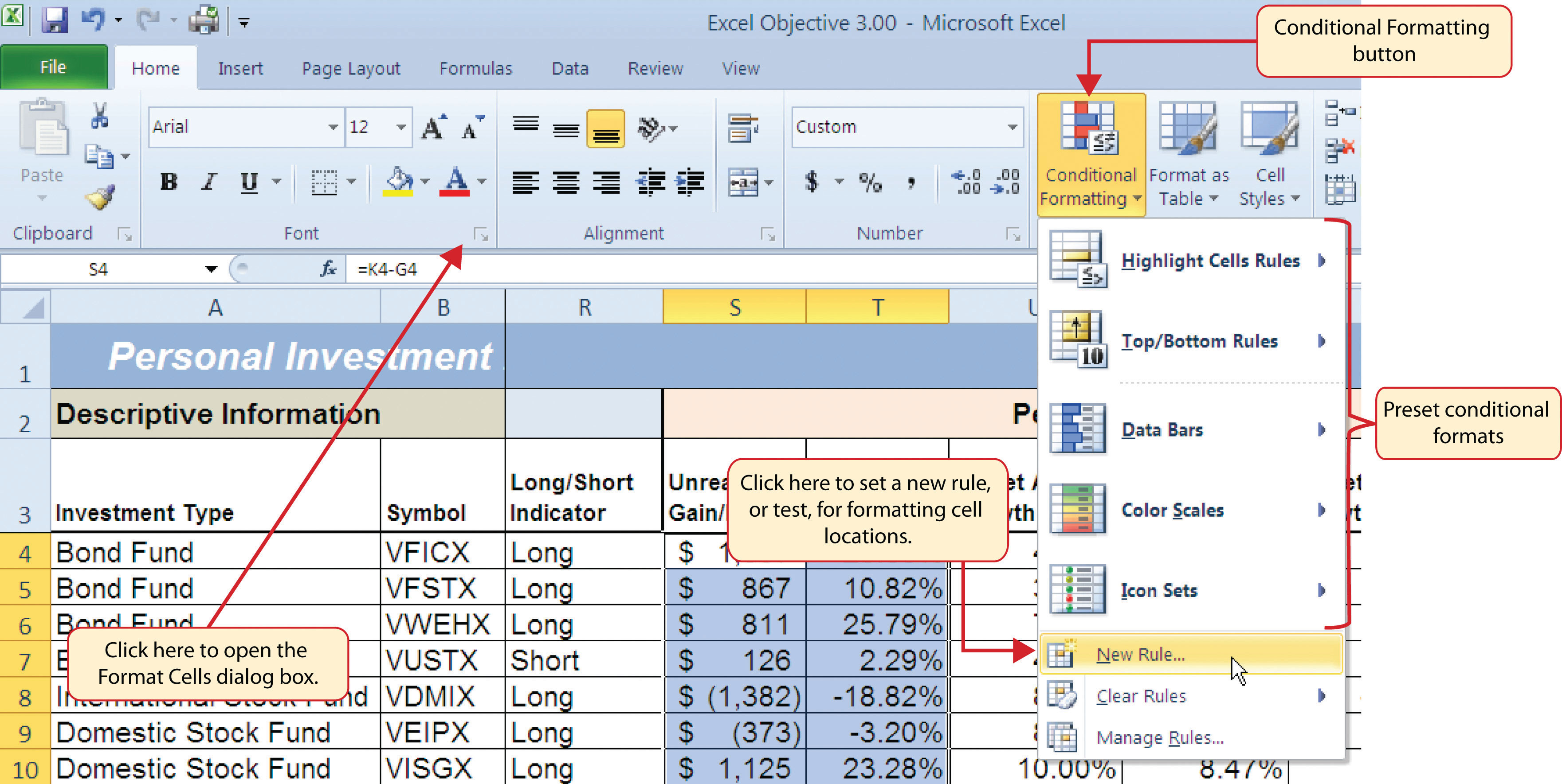
- At the top of the New Formatting Rule dialog box, you will find a list of options under the Select a Rule Type heading. Click the second option that states “Format only cells that contain.”
- In the lower portions of the New Formatting Rule dialog box, you will see several drop-down boxes under the heading Edit the Rule Description. Make sure the first drop-down box is set to Cell Value.
- Click the second drop-down box in the Edit the Rule Description section of the New Formatting Rule dialog box and select the “less than” option.
- Click in the input box, which is next to the drop-down box that was set in the previous step, and type a zero. This completes the logical test of the conditional format, which is going to evaluate if the value in any of the cells in the range S4:T18 is less than zero.
- Click the Format button, which is near the bottom of the New Formatting Rule dialog box. This will open the Format Cells dialog box.
- Click the drop-down box in the Color section of the Format Cells dialog box and select the red square from the color palette (see Figure 3.22 "Format Cells Dialog Box").
- Click the OK button at the bottom of the Format Cells dialog box.
- Click the OK button at the bottom of the New Formatting Rule dialog box. This completes the Conditional Formatting rule that will be applied to cells in the range S4:T18.
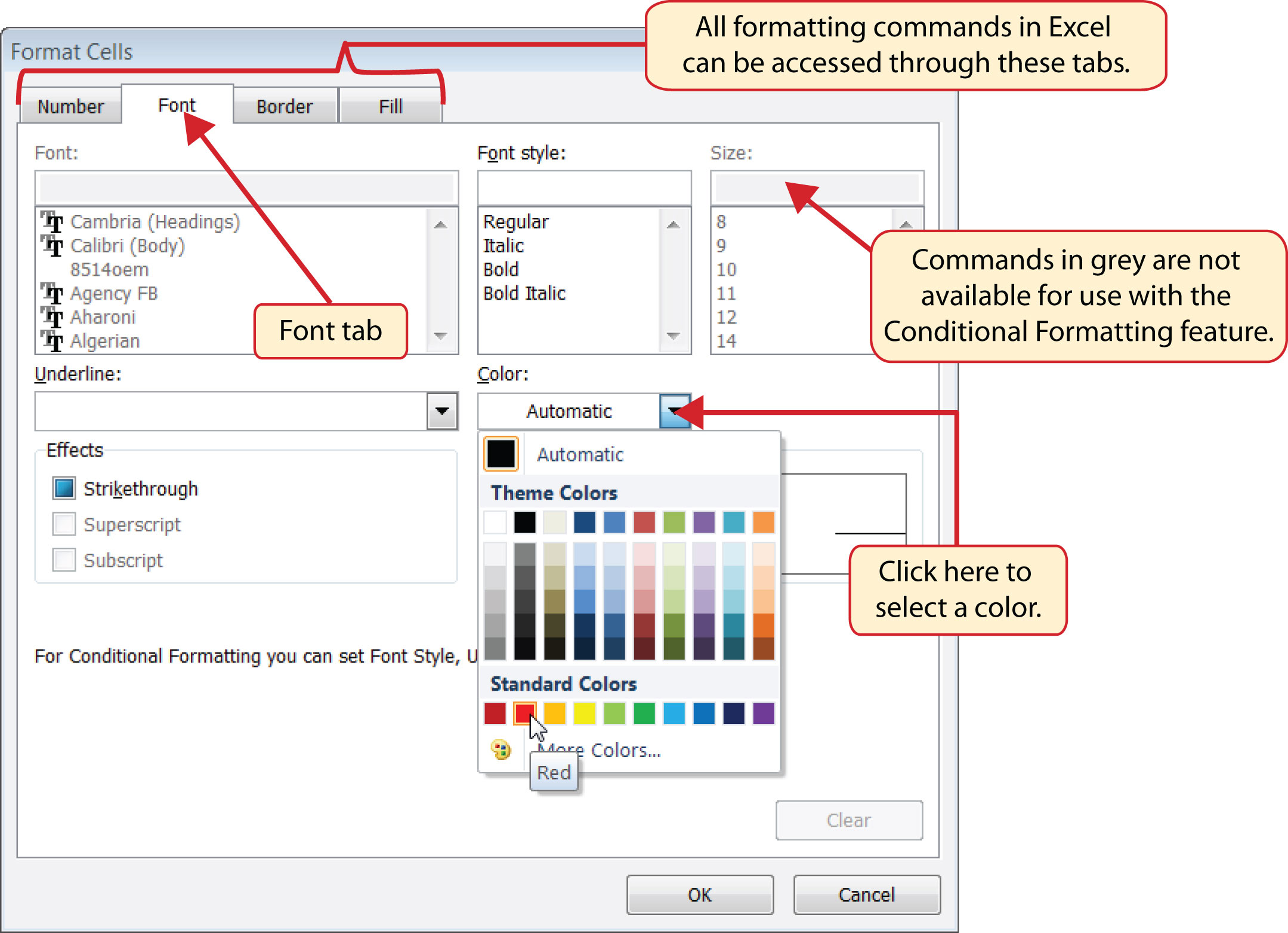
Figure 3.22 "Format Cells Dialog Box" shows the Format Cells dialog box. This opens when the Format button is clicked on the New Formatting Rule dialog box. Notice the tabs running across the top of the dialog box. All formatting features in Excel are grouped by category, which can be accessed by clicking the related tab on the Format Cells dialog box. You will see some of the formatting commands in light grey. This indicates that these commands cannot be used with the Conditional Formatting feature. You can use the Format Cells dialog box to apply any formatting features by clicking the Format Cells dialog button on the Home tab of the Ribbon (see Figure 3.21 "Conditional Formatting Options List").
Figure 3.22 Format Cells Dialog Box
Mouseless Commands
Open the Format Cells Dialog Box
- Hold down the CTRL key while pressing the SHIFT key and the letter F key on your keyboard.
Figure 3.23 "New Formatting Rule Dialog Box" shows the final settings for the New Formatting Rule dialog box. It is important to note that the “Format only cells that contain” option was selected in the New Formatting Rule dialog box to set a basic logical test that can be used to apply formatting commands automatically based on the values in cell locations.
Figure 3.23 New Formatting Rule Dialog Box
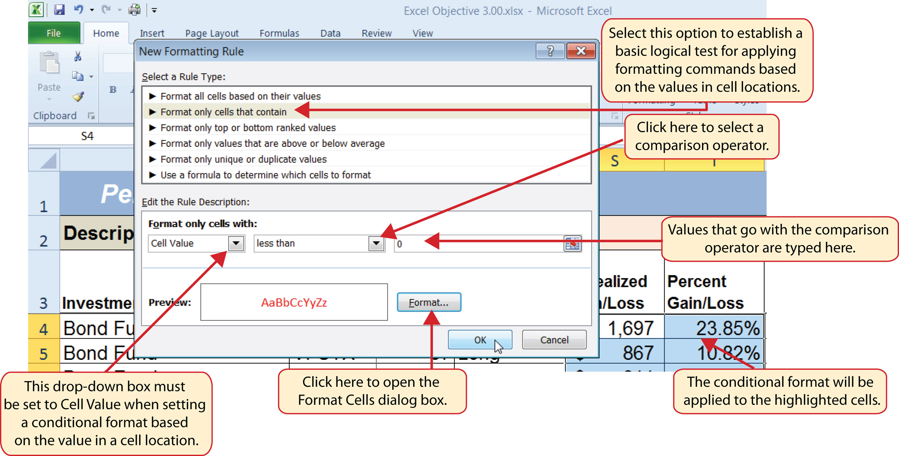
Figure 3.24 "Conditional Format Applied to the Range S4:T18" shows the results of the conditional formatting rule that was applied to the range S4:T18. Notice the font color is automatically changed to red for negative numbers.
Figure 3.24 Conditional Format Applied to the Range S4:T18
Skill Refresher: Conditional Formats (Cell Values)
- Click a cell or highlight a range of cells where the conditional format will be applied.
- Click the Home tab of the Ribbon.
- Click the Conditional Formatting button.
- Click the New Rule option from the drop-down list.
- Click the “Format only cells that contain” rule type from the list at the top of the New Formatting Rule dialog box.
- Select the type of contents you are evaluating in the first drop-down box near the bottom of the New Formatting Rule dialog box.
- Select a comparison operator description in the second drop-down box near the bottom of the New Formatting Rule dialog box.
- Enter a value in the input box next to the comparison operator box.
- Click the Format button to set the format that will be applied to the selected cell locations.
- Click the OK button at the bottom of the New Formatting Rule dialog box.
Key Takeaways
- The Freeze Panes command should be used to lock column and row headings in place while scrolling through large worksheets.
- The IF function is used to evaluate the contents of a cell location using a logical test. Based on the results of the logical test, you designate a custom output or calculation to be performed by the function.
- When using text, or nonnumeric data, to define any argument of the IF function, it must be placed inside quotation marks.
- A nested IF function is used when more than one logical test and more than two outputs are required for a project. Either the Value_if_true or the Value_if_false arguments can be defined with an IF function.
- When using percentages in any logical test or formula, you must use the percent symbol (%) or convert the percentage to a decimal. For example, 10% can also be expressed as .10.
- The OR function is used when many logical tests are required to evaluate the contents of a cell location. The OR function will produce a TRUE output if one of the logical tests is true.
- The AND function is used when many logical tests are required to evaluate the contents of a cell location. The AND function will produce a TRUE output if all of the logical tests are true.
- To minimize the complexity of nested IF functions, the OR and AND functions should be used when possible to define the logical_test argument of the IF function.
Exercises
-
Assume the value in cell B12 is 25. Any value greater than or equal to 25 is OK, and any value below 25 is too low. Which of the following IF functions will provide an accurate result?
- =IF(B12>25,OK,TOO LOW)
- =IF(B12>25, “TOO LOW”, “OK”)
- =IF(B12=25 OR B12>25, “OK”, “TOO LOW”)
- =IF(B12>=25, “OK”, “TOO LOW”)
-
Assume the value in cell C4 is 5 and the value in D4 is 2. If the value in C4 is greater than 10, or if the value in D4 is greater than or equal to 2, the output should read OK. Otherwise, the output should read LOW. Which of the following IF functions will provide an accurate result?
- =IF(C4>10 or D4>2 or D4=2, “OK”, “LOW”)
- =IF(OR(C4>10,D4>2,=2)=TRUE, “OK”, “LOW”)
- =IF(OR(D4>=2,C4>10)=TRUE, “OK”, “LOW”)
- =IF(C4>10, D4>=2, “OK”, “LOW”)
-
Assume the value in cell A2 is 0 and the value in B2 is 1%. If the value in A2 is equal to 0 and the value in B2 is greater than 1%, then the output of the function should be OK. Otherwise, the output of the function should be REBAL. Which of the following IF functions will provide an accurate result?
- =IF(A2=0, “OK”,IF(B2>1%, “OK”, “REBAL”))
- =IF(AND(A2=0,B2>1)=TRUE, “OK”, “REBAL”)
- =IF(AND(A2=0,B2>.01)=TRUE, “OK”, “REBAL”)
- Both a and c are correct.
-
Assume the value in cell E3 is 5. If the value in cell E3 is less than 0, the font color of the text should be red. If the value in cell E3 is greater than or equal to 0, the font color should remain black. When establishing a conditional format for cell E3, which rule type should be selected in the New Formatting Rule dialog box?
- Format all cells based on their values
- Format only cells that contain
- Format only top or bottom ranked values
- Use a formula to determine which cells to format