This is “Chapter Assignments and Tests”, section 1.5 from the book Using Microsoft Excel (v. 1.0). For details on it (including licensing), click here.
For more information on the source of this book, or why it is available for free, please see the project's home page. You can browse or download additional books there. To download a .zip file containing this book to use offline, simply click here.


1.5 Chapter Assignments and Tests
To assess your understanding of the material covered in the chapter, please complete the following assignments.
Careers in Practice (Skills Review)
Basic Monthly Budget for Medical Office (Comprehensive Review)
Starter File: Chapter 1 CiP Exercise 1
Difficulty: Level 1
Creating and maintaining budgets are common practices in many careers. Budgets play a critical role in helping a business or household control expenditures. In this exercise you will create a budget for a hypothetical medical office while reviewing the skills covered in this chapter. Begin the exercise by opening the file named Chapter 1 CiP Exercise 1.
Entering, Editing, and Managing Data
- Activate all the cell locations in the Sheet1 worksheet by left clicking the Select All button in the upper left corner of the worksheet.
- In the Home tab of the Ribbon, set the font style to Arial and the font size to 12 points.
- Increase the width of Column A so all the entries in the range A3:A8 are visible. Place the mouse pointer between the letter A and letter B of Column A and Column B. When the mouse pointer changes to a double arrow, left click and drag it to the right until the character width is 18.00.
- Enter Quarter 1 in cell B2.
- Use AutoFill to complete the headings in the range C2:E2. Activate cell B2 and place the mouse pointer over the Fill Handle. When the mouse pointer changes to a black plus sign, left click and drag it to cell E2.
- Increase the width of Columns B, C, D, and E to 10.14 characters. Highlight the range B2:E2 and click the Format button in the Home tab of the Ribbon. Click the Column Width option, type 10.14 in the Column Width dialog box, and then click the OK button in the Column Width dialog box.
- Enter the words Medical Office Budget in cell A1.
- Insert a blank column between Columns A and B. Activate any cell location in Column B. Then, click the drop-down arrow of the Insert button in the Home tab of the Ribbon. Click the Insert Sheet Columns option.
- Enter the words Budget Cost in cell B2.
-
Adjust the width of Column B to 13.29 characters.
Formatting and Basic Charts
- Merge the cells in the range A1:F1. Highlight the range and click the Merge & Center button in the Home tab of the Ribbon.
- Make the following format adjustments to the range A1:F1: bold; italics; change the font size to 14 points; change the cell fill color to Aqua, Accent 5, Darker 50%; and change the font color to white.
- Increase the height of Row 1 to 24.75 points.
- Center the title of the worksheet in the range A1:F1 vertically. Activate the range and then click the Middle Align button in the Home tab of the Ribbon.
- Make the following format adjustment to the range A2:F2: bold; and change the cell fill color to Tan, Background 2, Darker 10%.
- Set the alignment in cell B2 to Wrap Text. Activate the cell location and click the Wrap Text button in the Home tab of the Ribbon.
- Copy cell C3 and paste the contents into the range D3:F3.
- Copy the contents in the range C6:C8 by highlighting the range and clicking the Copy button in the Home tab of the Ribbon. Then, highlight the range D6:F8 and click the Paste button in the Home tab of the Ribbon.
- Calculate the total budget for all four quarters for the salaries. Activate cell B3 and click the down arrow on the AutoSum button in the Formulas tab of the Ribbon. Click the Sum option from the drop-down list. Then, highlight the range C3:F3 and press the ENTER key on your keyboard.
- Copy the contents of cell B3 and paste them into the range B4:B8.
- Format the range B3:F8 with a US dollar sign and zero decimal places.
- Sort the data in the range A2:F8 based on the values in the Quarter 4 column in ascending order. Highlight the range A2:F8 and click the Sort button in the Data tab of the Ribbon. Select Quarter 4 in the “Sort by” drop-down box and select Smallest to Largest in the Order drop-down box. Click the OK button.
- Add vertical and horizontal lines to the range A1:F8. Highlight the range and click the down arrow next to the Borders button in the Home tab of the Ribbon. Select the All Borders option from the drop-down list.
- Change the name of the Sheet1 worksheet tab to “Budget.” Double click the worksheet tab, type the word Budget, and press the ENTER key.
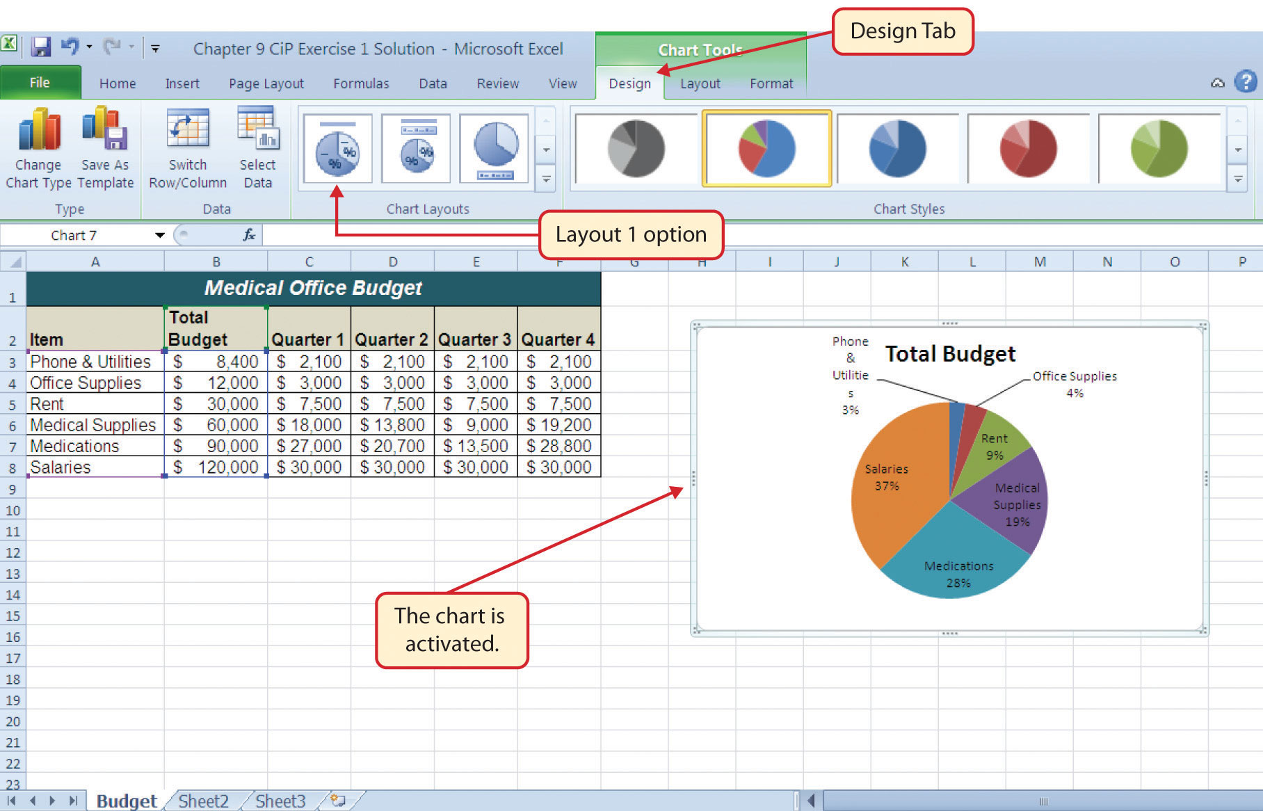
- Insert a pie chart using the data in the range A2:B8. Highlight the range and click the Pie button in the Insert tab of the Ribbon. Click the first option on the list (the Pie option).
- Click and drag the chart so the upper left corner is in the center of cell H2.
-
Add labels to the chart by clicking the Layout 1 option from the Chart Layouts list in the Design tab of the Ribbon. Make sure the chart is activated by clicking it once before you look for the Layout 1 Chart Layout option.
Printing
- Change the orientation of the Budget worksheet so it prints landscape instead of portrait.
- Adjust the appropriate settings so the Budget worksheet prints on one piece of paper.
- Add a header to the Budget worksheet that shows the date in the upper left corner and your name in the center.
- Add a footer to the Budget worksheet that shows the page number in the lower right corner.
- Use the Save As command in the File tab of the Ribbon to save the workbook by adding your name in front of the current workbook name (i.e., “your name Chapter 1 CiP Exercise 1”).
- Close the workbook and Excel.
Figure 1.66 Completed Medical Budget Exercise
Marketing for Specialty Women’s Apparel
Starter File: Chapter 1 CiP Exercise 2
Difficulty: Level 2
A key activity for marketing professionals is to analyze how population demographics change in certain regions. This is especially important for specialty retail stores that target a specific age group within a population. This exercise utilizes the skills covered in this chapter to analyze hypothetical population trends. The decisions that can be made with such information include where to open new stores, whether existing stores should be closed and reopened in other communities, or whether the product assortment should be adjusted. The purpose of this exercise is to use the skills presented in this chapter to analyze hypothetical population trends for a fashion retailer.
- In the Sheet1 worksheet, enter the year 2008 into cell B3.
- Use AutoFill to fill the years 2009 to 2012 in the range C3:F3.
- Change the font style to Arial and the font size to 12 points for all cell locations in the Sheet1 worksheet.
- Merge and center the cells in the range A1:F1.
- Make the following formatting adjustments to the range A1:F1: bold; italics; change the cell fill color to Olive Green, Accent 3, Lighter 60%; change the font size to 14 points.
- Enter the title for this worksheet into the range A1:F1 on two lines. The first line should read Population Trends by Age Group. The second line should read for Region 5.
- Increase the height of Row 1 so the title is visible.
- Delete Row 2.
- Increase the height of Row 2 to 21 points.
- Format the values in the range B3:F6 so a comma separates each thousands place with zero decimal places.
- Make the necessary adjustments to remove any pound signs (####) that may have appeared after formatting the values.
- Sort the data in the range A2:F6 based on the values in the year 2008 from largest to smallest.
- Enter the word Totals in cell A7.
- Increase the height of Row 7 to 22.50 points.
- Format the range A7:F7 so entries are bold and italic.
- In cell B7, add a total that sums the values in the range B3:B6. Format the value with zero decimal places and a comma for each thousands place.
- Copy the contents of cell B7 and paste them into the range C7:F7.
- Add vertical and horizontal lines to the range A1:F7.
- Add a very bold orange border around the perimeter of the range A1:F7.
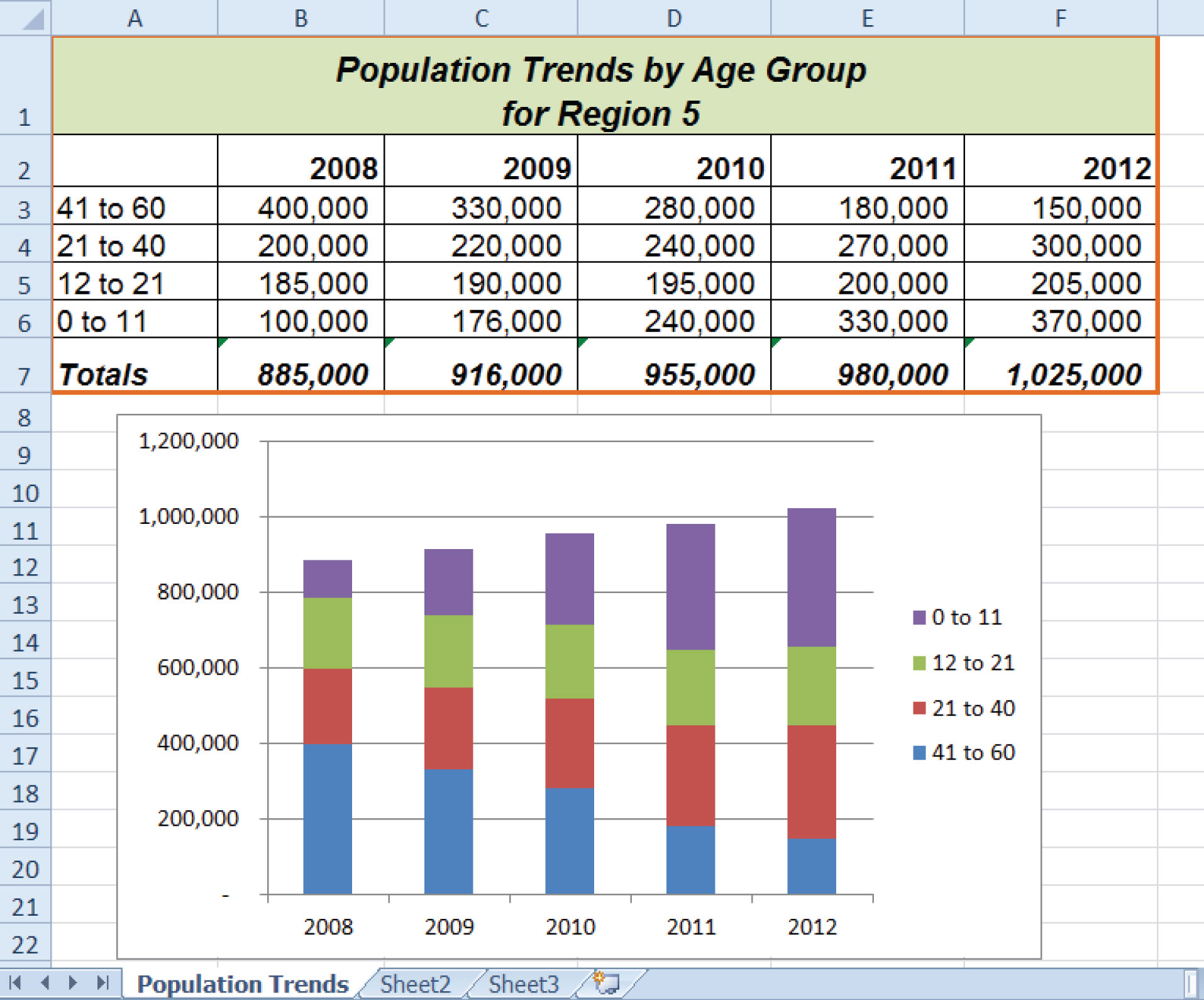
- Insert a column chart using the data in the range A2:F6. Select the 2-D Stacked Column format.
- Move the column chart so the upper left corner is in the middle of cell A8.
- Rename the Sheet1 worksheet tab to Population Trends.
- Adjust the appropriate settings so the Population Trends worksheet prints on one piece of paper.
- Add a header to the Population Trends worksheet that shows the date in the upper left corner and your name in the center.
- Save the workbook by adding your name in front of the current workbook name (i.e., “your name Chapter 1 CiP Exercise 2”). (Hint: you will need to Save As.)
- Close the workbook and Excel.
Figure 1.67 Completed Population Trends Exercise
Integrity Check
Starter File: Chapter 1 IC Exercise 1
Difficulty: Level 3
The purpose of this exercise is to analyze a worksheet to determine whether there are any integrity flaws. First, read the scenario below. Then, open the file that is related to this exercise and analyze the worksheets contained in the workbook. You will find a worksheet in the workbook named AnswerSheet. This worksheet is to be used for any written responses required for this exercise.
Scenario
Your coworker provides you with sales data in an Excel workbook, which you intend to use for a sales strategy meeting with your boss. The workbook was attached to an e-mail with the following points stated in the message.
- The data represents the top-selling items for the company last year with respect to sales dollars.
- I received the data from an analyst in my department who insisted the cost data for each item was included. However, I don’t see it. You might have to manually enter this yourself. I included the cost for each item below.
- The original data I received is in Sheet1. I copied this data and pasted it into Sheet2. I thought you might like to see this sorted.
-
Cost per item data:
Item Cost Black Flat $35.00 Bracelet $30.00 Brown Pump $25.00 Daisy Print $40.00 Grey Stripe $110.00 Jersey Knit $80.00 Navy Pinstripe $125.00 Navy Wool $135.00 Quartz Watch $80.00 Sandal $45.00 Tan Trench $115.00 Topaz Ring $50.00
Assignment
- Analyze the data in this workbook carefully. Would you be comfortable using this data in a meeting with your boss? Use the AnswerSheet in this workbook to briefly list any concerns you have with this data.
- If it is necessary to enter the cost information, enter it in the Sheet1 worksheet. If not, state why in the AnswerSheet.
- Correct any problems and make any adjustments you think are appropriate to this workbook.
- Save the workbook by adding your name in front of the current workbook name.
Applying Excel Skills
The assignment in this section requires that you apply the skills presented in this chapter to achieve the stated objective. Read the assignment first and then open the file and complete the stated requirements. When you complete an assignment, save the file by adding your name in front of the current name of the workbook.
Starter File: Chapter 1 AES Assignment 1
Difficulty: Level 3
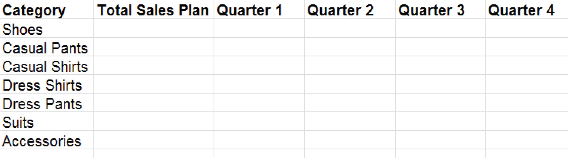
The workbook for this assignment contains sales plan data by month for merchandise categories sold by a hypothetical clothing retailer. Use the skills covered in this chapter to accomplish the points listed below.
- Show the total sales plan dollars next to each category in Column B.
-
Instead of showing the sales plan dollars by month, calculate the plan dollars for each quarter (see the following figure, “Layout for Sales by Quarter”). The months assigned to each quarter are as follows:
- Quarter 1: February, March, and April
- Quarter 2: May, June, and July
- Quarter 3: August, September, and October
- Quarter 4: November, December, and January
- Show the total plan for each quarter.
- Sort the merchandise categories based on the total sales plan dollars.
- Add any additional formatting enhancements that will make the worksheet easier to read.
Figure 1.68 Layout for Sales by Quarter
Chapter Skills Test
Starter File: Chapter 1 Skills Test
Difficulty: Level 2
Answer the following questions by executing the skills on the starter file required for this test. Answer each question in the order in which it appears. If you do not know the answer, skip to the next question. Open the starter file listed above before you begin this test.
- In the Sheet1 worksheet, enter the word Totals in cell C14.
- Format all the cells in Sheet1 to Arial font style and a 12-point font size.
- Set the character width for Columns A through G to 12.71.
- Edit the entry in cell B2 to read “Item Number.”
- Use AutoFill to fill the contents of cell B3 into the range B4:B13.
- Copy the contents of cell A3 and paste them into the range A4:A8.
- Delete Column F.
- Format the range A1:F2 so the text is Bold.
- Set the alignment in the range A2:F2 to Wrap Text.
- Change the fill color of the cells in the range A1:F1 to Red, Accent 2, Darker 25%.
- Make the following font changes to the range A1:F1: set the font color to white, add italics, and set the font size to 14.
- Merge and center the cells in the range A1:F1.
- Enter the title for this worksheet in the range A1:F1. The title should appear on two lines. The first line should read Status Report. The second line should read Sales and Inventory by Item.
- Increase the height of Row 1 so the entire title is visible.
- Insert a blank row above Row 14.
- Format the values in the range C3:C13 with a US dollar sign and two decimal places.
- Format the values in the range E3:F13 with zero decimal places and a comma at each thousands place.
- In cell E15, use AutoSum to calculate the sum of the values in the range E3:E14.
- Add vertical and horizontal lines to the range A1:F15.
- Add a bold line border around the perimeter of the range A1:F15.
- Insert a column chart using the data in the range D2:E13.
- Move the chart so the upper left corner is in the middle of cell H2.
- Sort the data in the range A2:F13 based on the values in the Sales in Units column. Sort the values in descending order or largest to smallest.
- Insert a new blank worksheet in the workbook.
- Delete Sheet3.
- Move Sheet4 ahead of Sheet2 so the order of the worksheets is Sheet1, Sheet4, and Sheet2.
- Rename the Sheet1 worksheet tab to “Status Report.”
- Change the orientation of the Status Report worksheet so it prints landscape instead of portrait.
- Adjust the appropriate settings so the Status Report worksheet prints on one piece of paper.
- Add a header to the Status Report worksheet that shows the date in the upper left corner and your name in the center.
- Add a footer to the Status Report worksheet that shows the page number in the lower right corner.
- Save the workbook by adding your name in front of the current workbook name (i.e., “your name Chapter 1 Skills Test”). (Hint: you will use Save As.)
- Close the workbook and Excel.