This is “Markup Pricing: Combining Marginal Revenue and Marginal Cost”, section 6.4 from the book Theory and Applications of Microeconomics (v. 1.0). For details on it (including licensing), click here.
For more information on the source of this book, or why it is available for free, please see the project's home page. You can browse or download additional books there. To download a .zip file containing this book to use offline, simply click here.


6.4 Markup Pricing: Combining Marginal Revenue and Marginal Cost
Learning Objectives
- What is the optimal price for a firm?
- What is markup?
- What is the relationship between the elasticity of demand and markup?
Let us review the ideas we have developed in this chapter. We know that changes in output lead to changes in both revenues and costs. Changes in revenues and costs lead to changes in profits (see Figure 6.16 "Changes in Revenues and Costs Lead to Changes in Profits"). We have a measure of how much revenues change if output is increased—called marginal revenue, which you can calculate if you know price and the elasticity of demand. We also have a measure of how much costs change if output is increased—this is called marginal cost. Given information on current marginal revenue and marginal cost, a marketing manager can then decide if a firm should change its price. In this section, we derive a rule that tells us how a manager should make this decision.
Figure 6.16 Changes in Revenues and Costs Lead to Changes in Profits
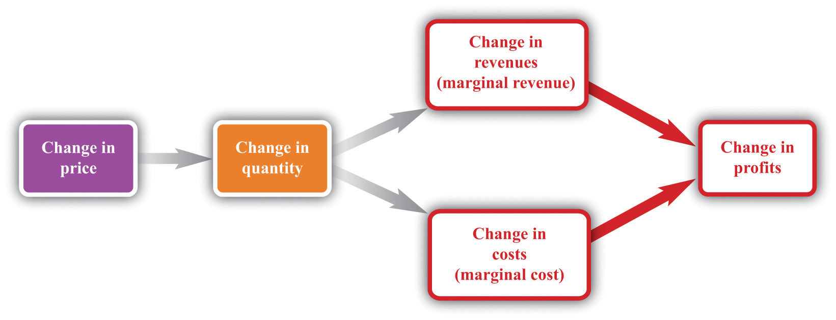
When a firm changes its price, this leads to changes in revenues and costs. The change in a firm’s profit is equal to the change in revenue minus the change in cost—that is, the change in profit is marginal revenue minus marginal cost. When marginal revenue equals marginal cost, the change in profit is zero, so a firm is at the top of the profit hill.
In the real world of business, firms almost always choose the price they set rather than the quantity they produce. Yet the pricing decision is easier to analyze if we think about it the other way round: a firm choosing what quantity to produce and then accepting the price implied by the demand curve. This is just a matter of convenience: a firm chooses a point on the demand curve, and it doesn’t matter if we think about it choosing the price and accepting the implied quantity or choosing the quantity and accepting the implied price (Figure 6.17 "Setting the Price or Setting the Quantity").
Figure 6.17 Setting the Price or Setting the Quantity
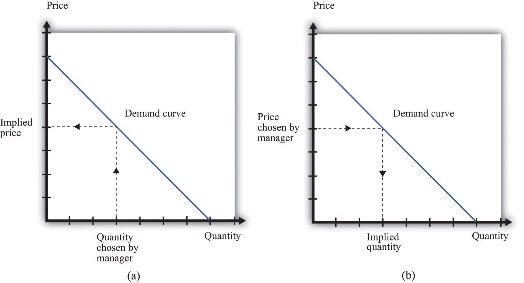
It doesn’t matter if we think about choosing the price and accepting the implied quantity or choosing the quantity and accepting the implied price
Suppose that a marketing manager has estimated the elasticity of demand, looked at the current price, and used the marginal revenue formula to discover that the marginal revenue is $5. This means that if the firm increases output by one unit, its revenues will increase by $5. The marketing manager has also spoken to her counterpart in operations, who has told her that the marginal cost is $3. This means it would cost an additional $3 to produce one more unit. From these two pieces of information, the marketing manager knows that an increase in output would be a good idea. An increase in output leads to a bigger increase in revenues than in costs. As a result, it leads to an increase in profits: specifically, profits will increase by $2. This tells the marketing manager that it is a good idea to increase output. From the law of demand, she should think about decreasing the price.
Figure 6.18 Optimal Pricing
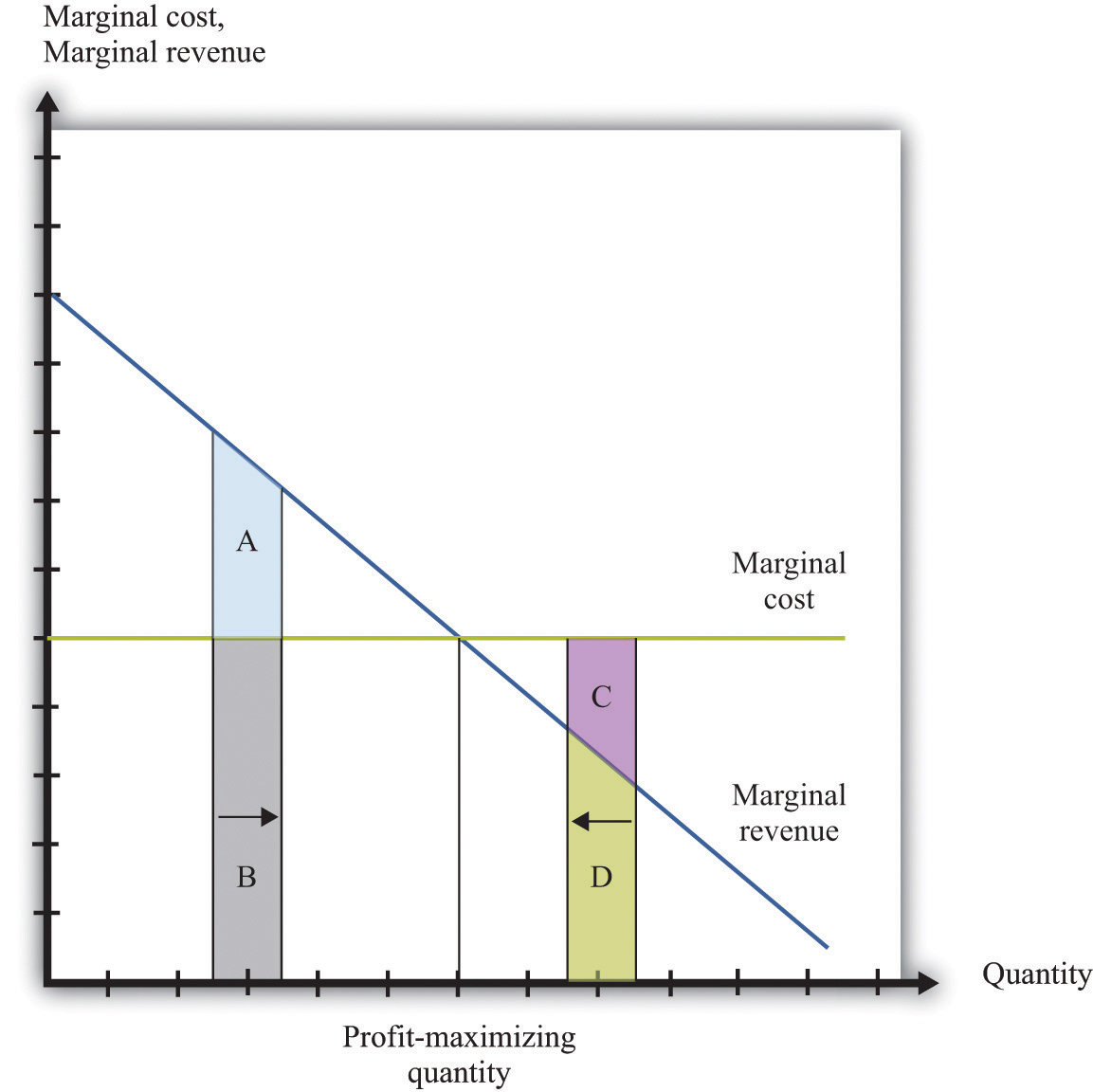
To the left of the point marked “profit-maximizing quantity,” marginal revenue exceeds marginal cost so increasing output is a good idea. The opposite is true to the right of that point.
Figure 6.18 "Optimal Pricing" shows this idea graphically. To the left of the point marked “profit-maximizing quantity,” marginal revenue exceeds marginal cost. Suppose a firm is producing below this level. If it increases its output, the extra revenue it obtains will exceed the extra cost. We see that an increase in output yields extra revenue equal to the areas A + B and extra costs equal to B. The increase in output yields extra profit, which is equal to A. Increasing its output is thus a good idea. Conversely, to the right of the profit-maximizing point, marginal revenue is less than marginal cost. If a firm reduces its output, the decrease in costs (C + D) exceeds the decrease in revenue (D). Decreases in output lead to increases in profit.
Profits are greatest when
marginal revenue = marginal cost.This is the point where a change in price leads to no change in profits, so we are at the very top of the profit hill that we drew in Figure 6.3 "The Profits of a Firm". See also Figure 6.17 "Setting the Price or Setting the Quantity".
The Markup Pricing Formula
Think about Ellie’s company. If it became more expensive for the company to produce each pill, it seems likely they would respond by raising their costs. Also, we said earlier that their customers are not very sensitive to changes in the price, which should allow them to set a relatively high price. In other words, the profit-maximizing price is related to the elasticity of demand and to marginal cost. These are the two critical ingredients of the pricing decision.
Toolkit: Section 17.15 "Pricing with Market Power"
Firms should set the price as a markup over marginal cost:This expression comes from combining the formula for marginal revenue and the condition that marginal revenue equals marginal cost. See the toolkit for more details.
and
There are three facts about markupThe percentage amount by which price exceeds marginal cost.:
- Markup is greater than or equal to zero—that is, the firm never sets a price below marginal cost.
- Markup is smaller when demand is more elastic.
- Markup is zero when the demand curve is perfectly elastic: −(elasticity of demand) = •.
Ellie’s team looked at their numbers. At the current price, −(elasticity of demand) = 1.47. They learned that the marginal cost was $0.28 per pill, and they were charging $0.50 per pill. Their current markup, in other words, was about 79 percent: 0.5 = (1+ 0.79) × 0.28. But if they applied the markup pricing formula based on the current elasticity of demand, they could charge a markup of 1/0.47 = 2.12—that is, more than a 200 percent markup, leading to a price of $0.87. It was clear that they could do better by increasing their price
A Pricing Algorithm
To summarize, a manager needs two key pieces of information when determining price:
- Marginal cost. We have shown that the profit-maximizing price is a markup over the marginal cost of production. If a manager does not know the magnitude of marginal cost, she is missing a critical piece of information for the pricing decision.
- Elasticity of demand. Once a manager knows marginal cost, she should then set the price as a markup over marginal cost. But this should not be done in an ad hoc manner; the markup must be based on information about the elasticity of demand.
Given these two pieces of information, a manager can then use the markup formula to determine the optimal price. Be careful, though. The markup formula looks deceptively simple, as if it can be used in a “plug-and-play” manner—given marginal cost and the elasticity of demand, plug them into the formula and calculate the optimum price. But if you change the price, both marginal cost and the elasticity of demand are also likely to change. A more reliable way of using this formula is in the algorithm shown in Figure 6.19 "A Pricing Algorithm", which is based on our earlier idea that you should find your way to the top of the profit hill. The five steps are as follows:
- At your current price, estimate marginal cost and the elasticity of demand.
- Calculate the optimal price based on those values.
- If the optimal price is greater than your actual price, increase your price. Then estimate marginal cost and the elasticity again and repeat the process.
- If the optimal price is less than your actual price, decrease your price. Then estimate marginal cost and the elasticity again and repeat the process.
- If the current price is equal to this optimal price, leave your price unchanged.
Figure 6.19 A Pricing Algorithm
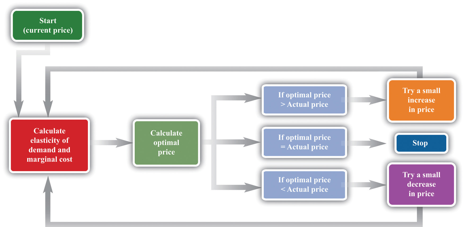
This pricing algorithm shows how to get the best price for a product.
Ellie’s team members were aware that, even though demand for the drug was apparently not very sensitive to price, they should not immediately jump to a much higher markup. They had found that based on current marginal cost and elasticity, the price could be raised. But as they raised the price, they knew that the elasticity of demand would probably also change. Looking more closely at their market research data, they found that at a price of $0.56 (a 100 percent markup), the elasticity of demand would increase to about 2. An elasticity of 2 means that the markup should be 100 percent to maximize profits. Thus—at least if their market research data were reliable—they knew that a price of $0.56 would maximize profits. Ellie recommended to senior management that the price of the drug be raised by slightly over 10 percent, from $0.50 per pill to $0.56 per pill.
Shifts in the Demand Curve Facing a Firm
So far we have looked only at movements along the demand curve—that is, we have looked at how changes in price lead to changes in the quantity that customers will buy. Firms also need to understand what factors might cause their demand curve to shift. Among the most important are the following:
- Changes in household tastes. Starting around 2004 or so, low-carbohydrate diets started to become very popular in the United States and elsewhere. For some companies, this was a boon; for others it was a problem. For example, companies like Einstein Bros. Bagels or Dunkin’ Donuts sell products that are relatively high in carbohydrates. As more and more customers started looking for low-carb alternatives, these firms saw their demand curve shift inward.
- Business cycle. Consider Lexus, a manufacturer of high-end automobiles. When the economy is booming, sales are likely to be very good. In boom times, people feel richer and more secure and are more likely to purchase a luxury car. But if the economy goes into recession, potential car buyers will start looking at cheaper cars or may decide to defer their purchase altogether. Many companies sell products that are sensitive to the state of the business cycle. Their demand curves shift as the economy moves from boom to recession.
- Changes in competitors’ prices. In a business setting, this is a critical concern. If a competitor decreases its price, this means that the demand curve you face will shift inward. For example, suppose that British Airways decides to decrease its price for flights from New York to London. American Airlines will find that its demand curve for that route has shifted inward. Ellie certainly has to worry about this because her company’s product has only a small number of competitors. A change in price of a competing blood pressure drug might make a big difference in the sales and profits of Ellie’s product.
If the demand curve shifts, should a firm change its price? The answer is yes if the shift in the demand curve also leads to a change in the elasticity of demand. In practice, this is likely to be the case, although it is certainly possible for a demand curve to shift without a change in the elasticity of demand. The correct response to a shift in the demand curve is to reestimate the elasticity of demand and then decide if a change in price is appropriate.
Complications
Pricing is a difficult and delicate job, and there are many factors that we have not yet considered:We address some of them in other chapters of the book; others are topics for more advanced classes in economics and business strategy.
- By far the most important problem that we have neglected is as follows: When making pricing decisions, firms may need to take into account how other firms will respond to their decisions. For example, a manager might estimate her firm’s elasticity of demand and marginal cost and determine that she could make more money by decreasing price. That calculation presumes that competing firms keep their prices unchanged. In markets with a small number of competitors, it is instead quite likely that other firms would respond by decreasing their prices. This would cause a firm’s demand curve to shift inward and probably leave it worse off than before.
- We have assumed throughout that a firm has to charge the same price for every unit that it sells. In many cases, this is an accurate description of pricing behavior. When a grocery store posts a price, that price holds for every unit on the shelf. But sometimes firms charge different prices for different units—by either charging different prices to different customers or offering individual units at different prices to the same customer. You have undoubtedly encountered examples. Firms sometimes offer quantity discounts, so the price is lower if you buy more units. Sometimes they offer discounts to certain groups of customers, such as cheap movie tickets for students. We could easily fill an entire chapter with other examples—some of which are remarkably sophisticated.
- Firms can have pricing strategies that call for the price to change over time. For example, firms sometimes engage in a strategy known as penetration pricing, whereby they start off by charging a low price in an attempt to develop or expand the market. Imagine that Kellogg’s develops a new breakfast cereal. It might decide to offer the cereal at a low price to induce people to try the product. Only after it has developed a group of loyal customers would it start setting their prices according to the markup principle.
- Pricing plays a role in the overall marketing and branding strategy of a firm. Some firms position themselves in the marketplace as suppliers of high-end offerings. They may choose to set high prices for their products to ensure that customers perceive them appropriately. Consider a luxury hotel that is contemplating setting a very low price in the off-season. Even though such a strategy might make sense in terms of its profits at that time, it might do long-term damage to the hotel’s reputation. For various reasons, customers often use the price of a product as an indicator of that product’s quality, so a low price can adversely affect a firm’s image.
- Psychologists who study marketing have found that demand is sensitive at certain price points. For example, if a firm increases the price of a product from $99.98 to $99.99, there might be very little effect on demand. But if the price increases from $99.99 to $100.00, there might be a much bigger effect because $100.00 is a psychological barrier. Such consumer behavior does not seem completely rational, but there is little doubt that it is a real phenomenon.
- Throughout this chapter, we have said that there is no difference between a firm choosing its price and taking as given the implied quantity or choosing its quantity and taking as given the implied price. Either way, the firm is picking a point on the demand curve. This is true, but there is a footnote that we should add. A firm’s demand curve depends on what its competitors are doing and, oddly enough, it does make a difference if those competitors are choosing quantities or prices.See Chapter 14 "Busting Up Monopolies" for discussion of this. We should also note that firms often do not know their demand curves with complete certainty. Suppose, for example, that the true demand curve for a firm’s product is actually further outward than a firm expects. If the firm sets the price, it will end up with an unexpectedly large quantity being demanded. If the firm sets the quantity, it will end up with an unexpectedly high price.
- We have focused our attention on the market power of firms as sellers, as reflected in the downward-sloping demand curves they face. Firms can also have market power as buyers. Walmart is such an important customer for many of its suppliers that it can use its position to negotiate lower prices for the goods it buys. Governments are also often powerful buyers and may be able to influence the prices they pay for goods and services. For example, government-run health-care systems may be able to negotiate favorable prices with pharmaceutical companies.
Key Takeaways
- At the profit-maximizing price, marginal revenue equals marginal cost.
- Markup is the difference between price and marginal cost, as a percentage of marginal cost.
- The more elastic the demand curve faced by a firm, the smaller the markup.
Checking Your Understanding
- We said that markup is always greater than zero. Look at the formula for markup. If markup is greater than zero, what must be true about −(elasticity of demand)? Can you see why this must be true? Look back at Figure 6.13 "Marginal Revenue and the Elasticity of Demand" for a hint.
- If price is a markup over marginal cost, then how does marginal revenue influence the pricing decision of a firm?
- Starting at the profit-maximizing price, if a firm increases its price, could revenue increase?