This is “The Monetary Transmission Mechanism”, section 10.2 from the book Theory and Applications of Macroeconomics (v. 1.0). For details on it (including licensing), click here.
For more information on the source of this book, or why it is available for free, please see the project's home page. You can browse or download additional books there. To download a .zip file containing this book to use offline, simply click here.
10.2 The Monetary Transmission Mechanism
Learning Objectives
After you have read this section, you should be able to answer the following questions:
- What is the link between the actions of the Fed and the state of the economy?
- What interest rate does the Fed target?
- What components of aggregate spending depend on the interest rate?
The actions of monetary authorities, such as the Fed and other central banks around the world, influence interest rates and thus the levels of employment, output, and prices. The links between a central bank’s actions and overall economic performance are far from straightforward, however. The process is summarized by the monetary transmission mechanismA mechanism explaining how the actions of a central bank affect aggregate economic variables, in particular real GDP. (shown in Figure 10.2 "The Monetary Transmission Mechanism"), which is the heart of this chapter. The monetary transmission mechanism is more than just some theory that economists have devised to try to make sense of monetary policy. It summarizes how the Fed thinks about its own actions.
Figure 10.2 The Monetary Transmission Mechanism
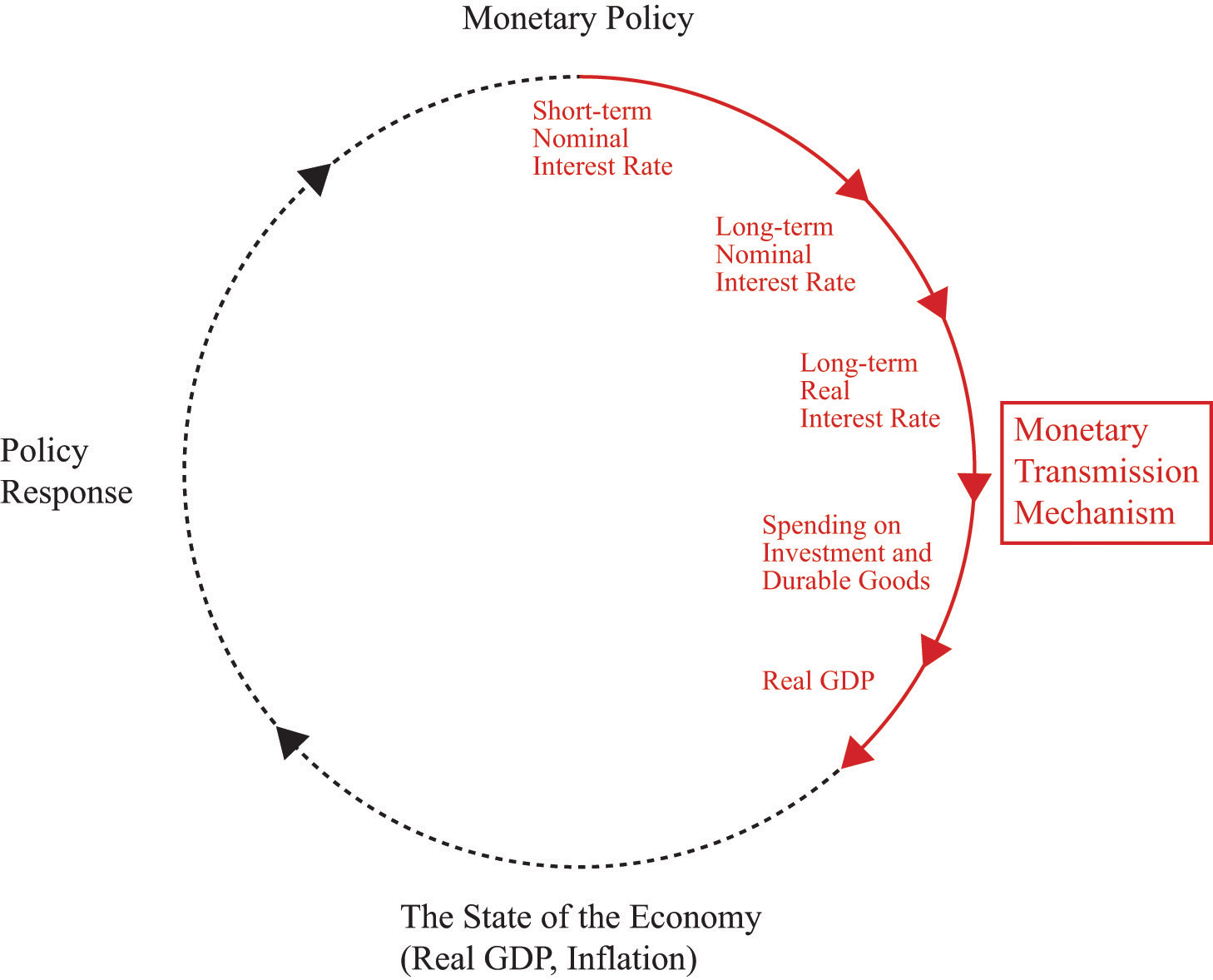
The Fed targets a short-term nominal interest rate. Changes in this rate lead to changes in long-term real interest rates, which affect spending on investment and durable goods, ultimately leading to a change in real GDP.
The monetary transmission mechanism explains how the actions of the Federal Reserve Bank affect aggregate economic variables, and in particular real gross domestic product (real GDP). More specifically, it shows how changes in the Federal Reserve’s target interest rate affect different interest rates in the economy and thus influence spending in the economy. Through open-market operations, the Fed targets a short-term nominal interest rateThe number of additional dollars that must be repaid for every dollar that is borrowed.. Changes in that interest rate in turn affect long-term nominal interest rates. Changes in long-term nominal rates lead to changes in long-term real interest ratesThe rate of return specified in terms of goods, not money.. Changes in long-term real interest rates affect investmentThe purchase of new goods that increase capital stock, allowing an economy to produce more output in the future. and durable goodsGoods that last over many uses. spending. Finally, changes in spending affect real GDP. We will examine every step of this process.
This chapter focuses on the effects of Fed actions, but essentially the same analysis applies to the study of monetary policy in other countries. The channels of influence are to a large degree independent of which country we study, although the magnitudes of the policy effects might differ across countries. Monetary policy differs across countries more through the targets set by different central banks than through the transmission mechanism.
How Well Can the Fed Meet Its Target?
On February 2, 2005, the Federal Open Market Committee (FOMC) decided to increase the target federal funds rate to 2.5 percent. The word target is critical here. If you listen to television news, you might get the impression that the Fed sets interest rates. It does not. It influences them, with greater or lesser success at different times.
Figure 10.3 "Target and Actual Federal Funds Rate, 1971–2005" shows the monthly target and actual federal funds rate between 1971 and 2008. From this picture, it is evident that the target and actual federal funds rates move together. We can conclude that the first stage of the monetary transmission mechanism is reliable. The Fed can influence the federal funds rate. So far so good—at least for this period of time. As we shall see later, when we consider more recent events, the Fed was much less successful in targeting the federal funds rate during the periods of financial distress in 2007 and 2008.
Figure 10.3 Target and Actual Federal Funds Rate, 1971–2005
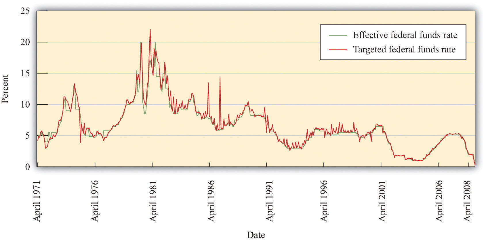
The target and actual federal funds rates move closely together.
From Short-Term Interest Rates to Long-Term Interest Rates
The next question is, do movements in the federal funds rate lead to corresponding movements in long-term interest rates? By “long-term,” we mean the rates on assets that have a maturity of at least 1 year and, in particular, assets that have a maturity of 5 years, 10 years, or even longer. ArbitrageThe act of buying and then selling an asset to take advantage of profit opportunities. among different assets means that annual interest rates on assets with different maturitiesThe term in which an asset comes due. are linked. As a result, the actions of the Fed to influence short-term rates also affect long-term rates.
Figure 10.4 "Short-Term and Long-Term Interest Rates" shows the relationship between the federal funds rate and longer-term interest rates. Broadly speaking, these long rates move with the federal funds rate. But it is also clear that the longer the horizon on the debt, the less responsive is the interest rate to movements in the federal funds rate.
This is one of the difficulties faced by the Fed: it can target short-term rates very accurately, but its influence on long-term rates is much less precise. Since—as we shall see—many economic decisions depend on long-term rates, the Fed’s ability to influence the economy is imperfect. Some writers have suggested that the Fed is an all-powerful organization that can move the economy around on a whim. There is no doubt that the Fed wields a great deal of power over the economy. Nevertheless, the Fed’s influence is substantially limited by the fact that it cannot control long-term interest rates with anything like the same precision that it brings to bear on the federal funds rate.
Figure 10.4 Short-Term and Long-Term Interest Rates
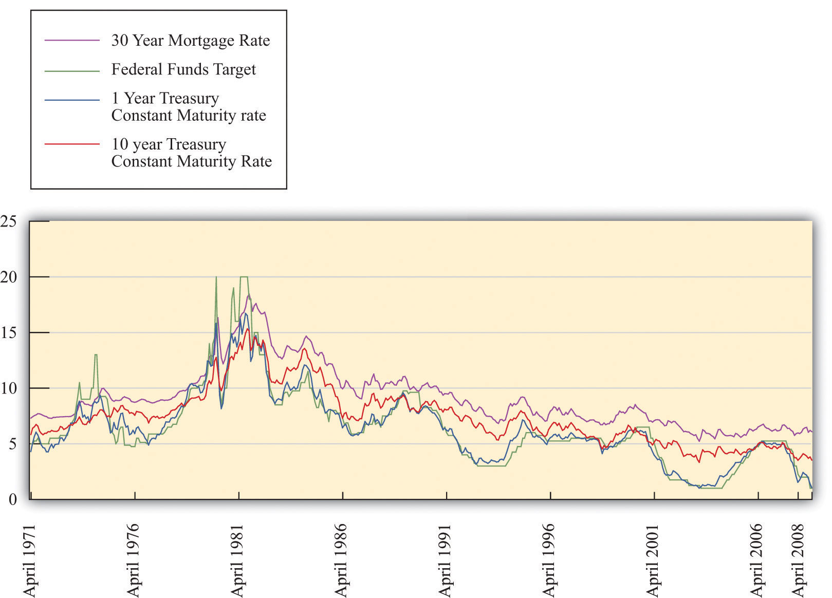
The Fed’s ability to influence long interest rates is much more limited than its ability to affect short rates.
From Nominal Interest Rates to Real Interest Rates
So far in this section, we have been considering nominal interest rates, but we know that the decisions of firms and households are based on real interest rates. The link between nominal and real interest rates is given by the Fisher equation:
real interest rate ≈ nominal interest rate − inflation rate.To use this relationship, we simply subtract the inflation rate from the nominal interest rate. So if the nominal interest rate were 15 percent, as it was in the early 1980s, and the inflation rate were 12 percent, then the real interest rate would be 3 percent. But if the inflation rate were higher—say, 18 percent—then the real interest rate would be minus 3 percent.
Toolkit: Section 16.14 "The Fisher Equation: Nominal and Real Interest Rates"
The toolkit reviews the derivation of the Fisher equation.
Figure 10.5 "Real and Nominal Interest Rates" shows the nominal and real rates of return for a one-year Treasury bond. Because inflation is positive, the nominal interest rate exceeds the real rate. The figure shows that the nominal and real rates typically move closely together. In the early 1980s, for example, the real interest rate was negative. Presumably when households lent money in the early 1980s, they did not expect a negative return on their saving but instead expected that the nominal interest rate would exceed the inflation rate. From that perspective, the negative real interest rate is a consequence of higher than anticipated inflation.
The Fed’s ability to influence longer-term nominal rates through its influence on the federal funds rate apparently extends to the real interest rate as well. The connection is not perfect, however. On some occasions, movements in nominal rates are decoupled from movements in real rates.
Figure 10.5 Real and Nominal Interest Rates
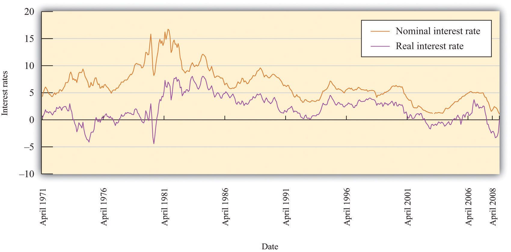
Changes in nominal interest rates generally lead to changes in real interest rates, but the link between the two is imperfect.
From Real Interest Rates to Spending on Durable Goods
Real rates of interest influence spending by both households and firms. The main categories of purchases that are affected by interest rates are as follows:
- Investment spending by firms
- Housing purchases by households
- Durable goods purchases by households
What do these have in common? In each case, the purchase yields a flow of benefits that extends over some significant period of time. If a firm builds a new factory or purchases a new piece of machinery, it typically expects to be able to use that plant and equipment for years or decades. When a household buys a new home, it expects either to live there for a long time or else to sell it to someone else who can live there. If you buy a durable good such as a new car or a refrigerator, you expect to obtain the benefits of that purchase for several years.
Figure 10.6 "Real Interest Rates and Spending on Durable Goods" shows the relationship between the real interest rate and spending on durable goods. The higher the real interest rate is, the lower is the amount of spending on durable goods. Of course, the relationship need not be a straight line; we have just drawn it this way for simplicity. As you might imagine, monetary policymakers are very interested in the exact form of this relationship. They want to know exactly how big a change in durable goods spending is likely to follow from a given change in interest rates.
Figure 10.6 Real Interest Rates and Spending on Durable Goods
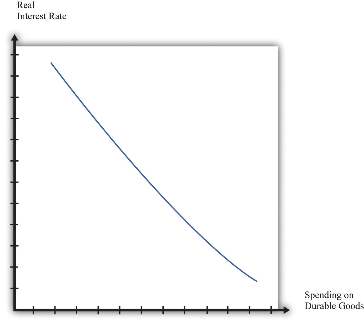
At higher interest rates, firms are less likely to borrow for investment projects, and households are less likely to borrow to purchase housing and durable goods such as new cars. Thus spending on durable goods is lower at higher interest rates and vice versa.
Discounted Present Value and Spending on Durable Goods
To understand in more detail why interest rates affect spending on durable goods, consider the purchase of a machine by a firm. Firms carry out such investment spending because they expect the machine to yield a flow of profits not only in the present but also for several years into the future. A machine is a capital good; it is used in the production of other goods and is not used up during the production process. The fact that the returns from the machine accrue over several years is what we mean by the term durable.
It is not correct to simply add profit flows in different years because a dollar today is usually worth more than a dollar next year. Why? If you take a dollar today and put it in a savings account at the bank, you will get your dollar plus interest back next year. If the interest rate is 10 percent, then $1 this year is worth $1.10 next year. Turning it around, $1 next year is worth only about 91 cents this year (because 1/1.1 = 0.91).
The technique for adding together flows of resources in different periods is called discounted present value. To work out whether a given investment is profitable, a firm must calculate the value, in today’s terms, of the flows of profits that it expects to receive. It then compares this to the cost of the investment. If the discounted present value of the profits exceeds the cost, the firm will undertake the investment.
Toolkit: Section 16.3 "Discounted Present Value"
You can review discounted present value in the toolkit.
Table 10.1 "Return on Investment" illustrates a simple investment decision. In year 1, you pay for a machine, and it yields some profit in that year. The next year, the machine yields further profit. Suppose you, as a manager of a firm, must decide whether or not to buy this machine. How do you make this decision? In the first year, you pay $970 for the machine and earn only $500 back, so you are down $470. In the second year, you will earn an additional $500—but you have to wait a year to get this money. Think of the profits in year 2 as being in real terms—that is, already corrected for inflation.
Table 10.1 Return on Investment
| Year | Payment for Machine | Real Profit from Machine |
|---|---|---|
| 1 | 970 | 500 |
| 2 | 0 | 500 |
To decide about the purchase of the machine, you need to know the interest rate. If the interest rate were zero, the calculation would be easy. You could just add together the profit flows in the 2 years, observe that $1,000 is more than the $970 that you have to pay for the machine, and conclude that the purchase is a good idea. Now suppose the real interest rate is 5 percent, which means that the real interest factor is 1.05. Then the discounted present value of the profit flows from the machine is given by the following equation:
In this case, the purchase is still a good idea. You will earn $976 in present value terms, exceeding the $970 that you have to pay, so you still come out ahead.
But what if that the real interest rate is 10 percent? In this case,
This is less than the amount that you had to pay for the machine. The investment no longer looks like a good idea. The higher the interest rate, the more we must discount future earnings, so the less likely it is that a current investment will be profitable.
In most real-life cases, the flow of profits extends for several years, so the discounted present value calculation is somewhat harder. (Still, even harder calculations can be done easily with a calculator or a spreadsheet.) Our example may be simple, but it illustrates our key point. As the real interest rate decreases, the discounted present value of profits from a machine increases. In the economy, there are at any given time many possible investment opportunities. Some have higher profit flows than others. At lower interest rates, more machines will be profitable to purchase: investment increases as the real interest rate decreases.
Households purchase homes and durable consumption goods, such as cars and household appliances. If the household borrows to make such purchases (through mortgages, car loans, or other personal loans), then exactly the same logic applies. Higher interest rates will tend to deter the household from these purchases, whereas lower interest rates will encourage purchases.Even if the household uses its own accumulated saving to buy the durable good, there is an opportunity cost of using these funds: it could have put the money in the bank instead. The higher the real interest rate, the better it looks to put money in the bank. Households usually have some choice about when exactly to purchase such goods. If interest rates are high this year, it probably makes sense to put off that purchase of a new washing machine until next year, when rates might be lower.
The effect of an increase in the real interest rate on spending on durable goods is captured in Figure 10.7 "The Relationship between the Real Interest Rate and Spending on Durable Goods".
Figure 10.7 The Relationship between the Real Interest Rate and Spending on Durable Goods
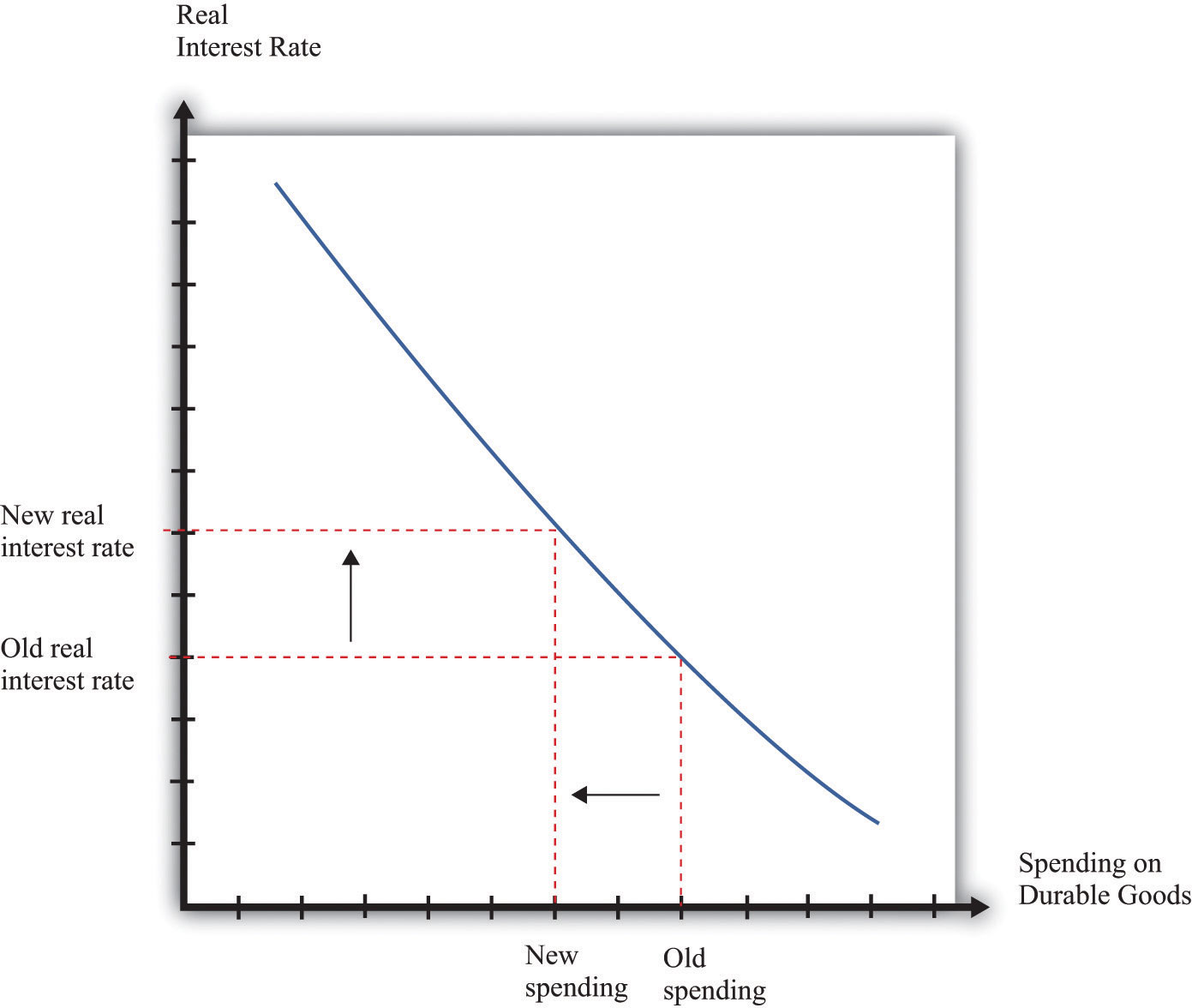
When the real interest rate increases, spending on durable goods decreases.
From Spending on Durable Goods to Real GDP
Look again at Figure 10.2 "The Monetary Transmission Mechanism". We have so far explored the links from the Fed’s decision on a target to spending on durable goods and net exports. Now we examine how changes in spending affect total output in the economy.
The aggregate expenditure model allows us to see how changes in aggregate spending translate into changes in GDP, at a given price level. The idea underlying the aggregate expenditure model is that, by the rules of national income accounting, real GDP must equal both production and spending. If spending increases, then it must be the case that production increases as well. The key diagram of the aggregate expenditure model is shown in Figure 10.8 "Aggregate Spending Depends Positively on Income".
Variations in the real interest rate influence the level of aggregate spending through the level of autonomous spending (the intercept term). To see why, recall that total spending is the sum of consumption, investment, government purchases, and net exports. The intercept term of the expenditure relationship includes all the influences on spending other than output. Thus any changes in consumption, investment, or net exports that are not induced by changes in output show up as changes in the intercept term. In particular, if an increase in interest rates causes firms to cut back on their investment spending, then the planned spending line shifts downward.
Figure 10.8 Aggregate Spending Depends Positively on Income
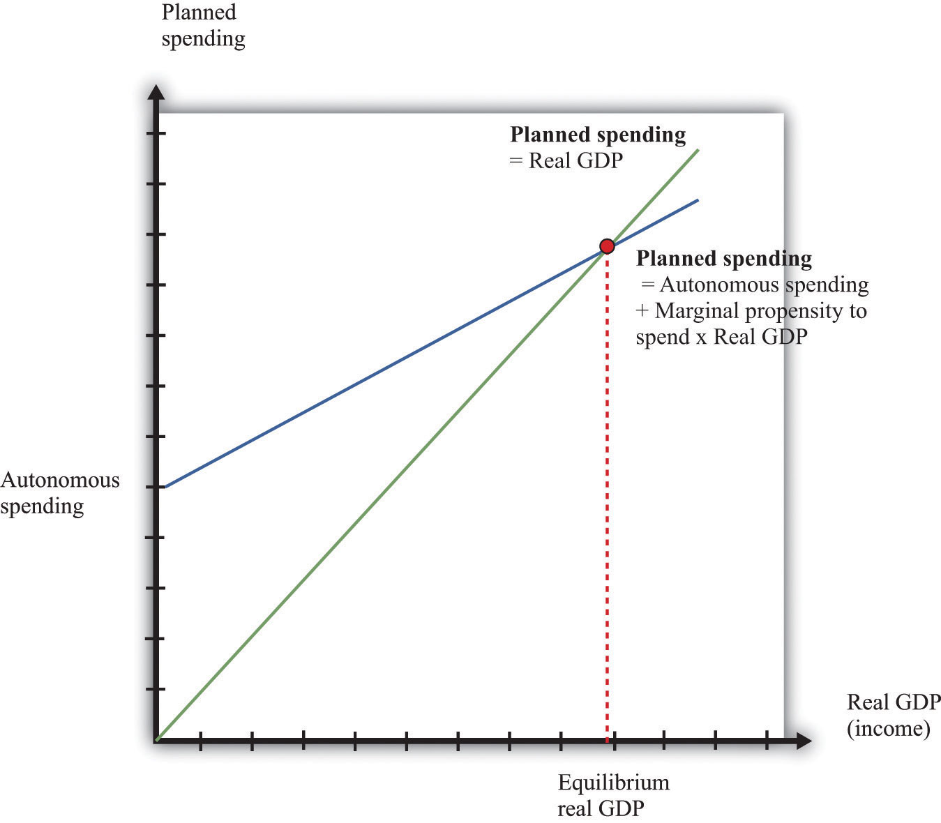
The economy is in equilibrium when spending equals real GDP.
We saw in Figure 10.7 "The Relationship between the Real Interest Rate and Spending on Durable Goods" that, as the real interest rate increases, the level of spending on durables decreases. This leads to a decrease in spending, given the level of income, and thus a decrease in the intercept of the spending line, as shown in Figure 10.9 "Increases in Real Interest Rates Reduce Real GDP". The magnitude of the reduction in spending—that is, the shift downward in the spending line—will depend on the sensitivity of durable spending to real interest rates. The more sensitive durable spending is to changes in the real interest rate, the larger the shift in the spending line will be when the real interest rate changes.
Figure 10.9 Increases in Real Interest Rates Reduce Real GDP
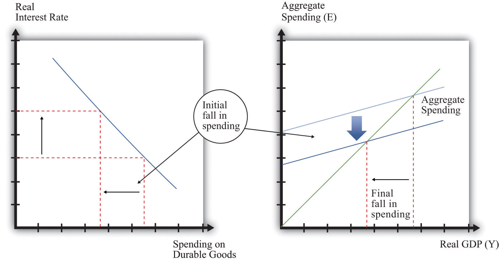
As a consequence of increases in real interest rates, aggregate spending decreases.
The initial reduction in spending induced by the increased real interest rate is then magnified by the multiplier process. The reduction in durable spending leads to a contraction in output. The resulting decrease in income leads households to spend less, leading to further contractions in output and income. In the end, the overall reduction in output exceeds the initial reduction in spending. This is visible in Figure 10.9 "Increases in Real Interest Rates Reduce Real GDP" from the fact that the horizontal difference between the old and new equilibrium points is larger than the vertical shift in the spending line.
Toolkit: Section 16.19 "The Aggregate Expenditure Model"
You can review the aggregate expenditure model and the multiplier in the toolkit.
The Real Interest Rate–Real GDP Line
We can summarize much of the monetary transmission mechanism by means of a relationship between real interest rates and real GDP, as shown in Figure 10.10 "The Relationship between the Real Interest Rate and Real GDP". After we work through all the connections from real interest rates to the various components of spending and real GDP, we find that there is a level of real GDP associated with each real interest rate. The higher the interest rate, the lower is real GDP.
Figure 10.10 The Relationship between the Real Interest Rate and Real GDP
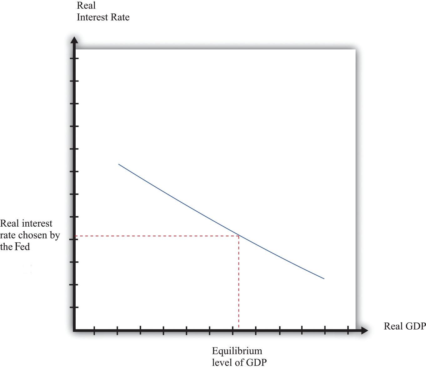
This picture summarizes several steps in the monetary transmission mechanism to show the relationship between real interest rates and real GDP.
As the monetary authority changes the real interest rate, the economy moves along this curve. So, for example, a reduction in the real interest rate leads to increased spending on durables, which, through the multiplierThe amount by which a change in autonomous spending must be multiplied to give the change in output, equal to 1 divided by (1 – the marginal propensity to spend). process, increases aggregate output. The shape of the curve tells us something about the Fed’s ability to influence the economy. Suppose that (1) durable spending is very sensitive to the real interest rate and (2) the multiplier is large; then imagine that the Fed cuts interest rates. Firms and households both respond to this change. Firms decide to carry out more investment: they buy new machinery, open new plants, and so forth. Households, attracted by the low interest rates, borrow to buy new cars and new homes. As a result, durable spending increases substantially. Furthermore, this increase in spending leads to higher income and thus to further increases in spending by households. The end result is a large increase in real GDP. In this case, the curve is flat.
Figure 10.11 The Fed’s Influence on the Economy Depends on the Real Interest Rate–Real GDP Relationship
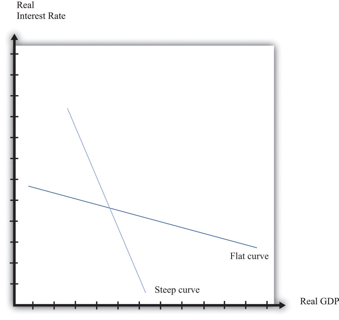
When the curve is flat, the Fed is able to have a big influence on the economy. When the curve is steep, it is harder for the Fed to affect economic activity.
Figure 10.11 "The Fed’s Influence on the Economy Depends on the Real Interest Rate–Real GDP Relationship" shows both this case and the case where it is harder for the Fed to influence the economy. If spending on durable goods is not very responsive to changes in the real interest rate and the multiplier is small, then changes in interest rates end up having only a small effect on real GDP. In the diagram, this shows up as a steep curve. The Fed’s ability to use the monetary transmission mechanism to its advantage requires good knowledge of the shape of this relationship between interest rates and output.
Key Takeaways
- The monetary transmission mechanism describes the links between the actions of the Fed and the state of the aggregate economy.
- The Fed targets a short-term nominal interest rate called the federal funds rate. The Fed does not set this rate directly but rather uses its tools to influence this interest rate.
- The main components of spending that depend on the real interest rate are spending by households on durable goods and investment. When these components of spending are sensitive to the interest rate, then the Fed can influence the economy through small variations in its target federal funds rate.
Checking Your Understanding
- Which interest rate determines investment spending—the real interest rate or the nominal interest rate?
- Some newspapers state that the Fed sets the interest rate. Is that right?


