This is “The Reagan Tax Cut”, section 27.4 from the book Theory and Applications of Economics (v. 1.0). For details on it (including licensing), click here.
For more information on the source of this book, or why it is available for free, please see the project's home page. You can browse or download additional books there. To download a .zip file containing this book to use offline, simply click here.


27.4 The Reagan Tax Cut
Learning Objectives
After you have read this section, you should be able to answer the following questions:
- What was the state of the economy at the time of the Reagan tax cut?
- What framework was used for analyzing the effects of this tax cut?
- What were the effects of the tax cut?
When Ronald Reagan was elected US president in 1980, the US economy was not in very good shape. The 1970s had been a very difficult time for economies throughout the world. The oil-producing nations of the world, acting as a cartel, had increased oil prices substantially, and, as a result, energy costs had increased. These energy prices triggered a severe recession in the mid 1970s and a smaller recession in the late 1970s. Figure 27.8 "Real GDP in the 1970s" shows the US real gross domestic product (GDP) for this period. As well as recessions, the United States was suffering from inflation that was very high by historical standards: prices were increasing by more than 10 percent a year.
Figure 27.8 Real GDP in the 1970s
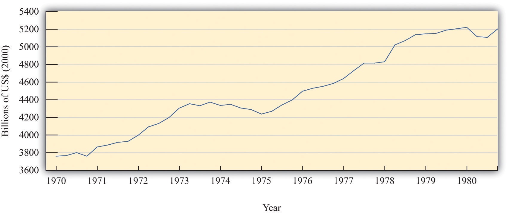
The figure shows real GDP in the 1970s. There was a protracted recession in the mid-1970s and a smaller recession toward the end of the decade.
Source: Bureau of Economic Analysis.
President Reagan and his economic advisors argued that high taxes were one of the causes of the relatively poor performance of the US economy. In particular, they claimed that taxes on income were deterring people from working as hard as they would otherwise. Unlike President Kennedy’s advisors, who had argued that income tax cuts would increase real GDP by stimulating aggregate expenditure, Reagan’s advisors said that tax cuts would increase potential output. Proponents of this economic view became known as supply siders because their focus was on the production of goods and services rather than the amount of spending on goods and services.
After his inauguration, President Reagan pushed hard for changes in the tax code, and Congress enacted the Economic Recovery Tax Act (ERTA) in 1981. This law reduced tax rates substantially: Figure 27.9 "Marginal and Average Tax Rates, 1982 to 1984" shows marginal and average tax rates for 1982, 1983, and 1984. The marginal tax rates are shown in part (a) in Figure 27.9 "Marginal and Average Tax Rates, 1982 to 1984": marginal rates decreased significantly for taxable income up to about $80,000.In contrast to Figure 27.3, no tax was payable until taxable income was $2,300. This is because the definition of taxable income at that time included the exemption. As a consequence, average tax rates also decreased significantly between 1982 and 1984 (part (b) in Figure 27.9 "Marginal and Average Tax Rates, 1982 to 1984").
Figure 27.9 Marginal and Average Tax Rates, 1982 to 1984
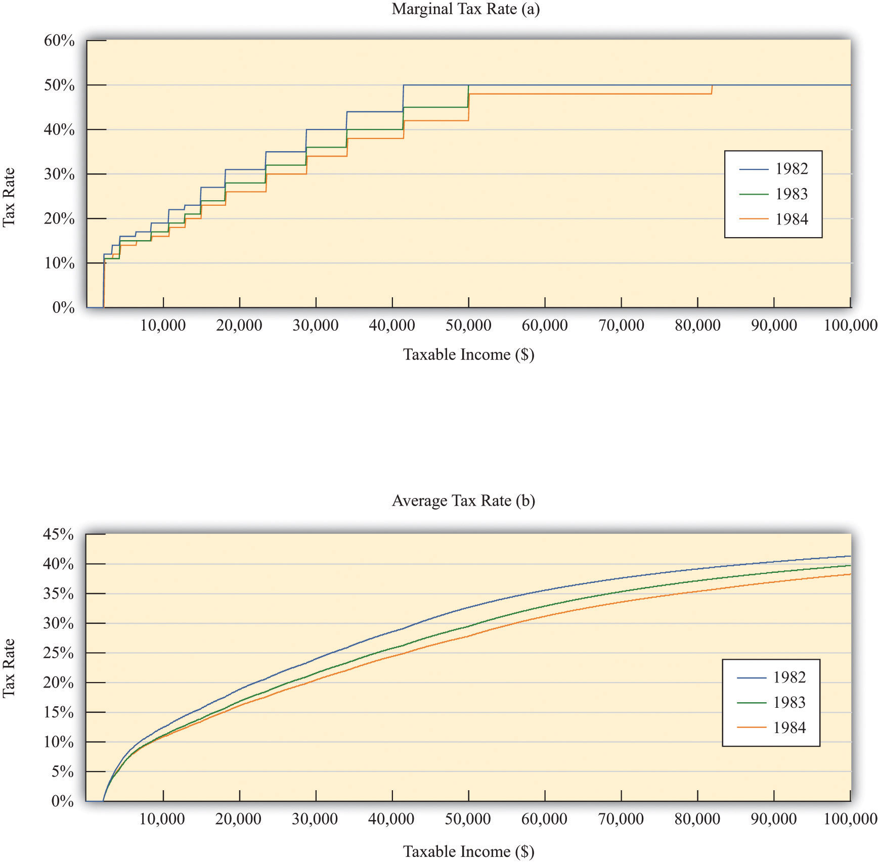
The figure shows marginal (a) and average (b) tax rates from 1982 to 1984, the period of the Reagan tax cuts. Both marginal and average rates decreased substantially.
Source: Department of the Treasury, IRS 1987, “Tax Rates and Tables for Prior Years” Rev 9-87
The main mechanism that the supply siders proposed was that lower income taxes would increase the incentive to work. To analyze this claim, we need to investigate how the decision to supply labor depends on income taxes. As with our analysis of consumption, we look at labor supply by thinking about the behavior of a single household. We then suppose that the household can be taken as representative of the entire economy.
Labor Supply
Each individual faces a time constraint: there are only 24 hours in the day, which must be divided between working hours and leisure hours. An individual’s time budget constraintThe restriction that the sum of the time you spend on all your different activities must be exactly 24 hours each day. says that, on a daily basis,
leisure hours + working hours = 24 hours.The labor supply decision is equivalently the decision about how much leisure time to enjoy. This decision is based on the trade-off between enjoying leisure and working to purchase consumption goods. People like having leisure time, and they prefer more leisure to less. Leisure can be thought of as a “good,” just like chocolate or blue jeans or cans of Coca-Cola. People sacrifice leisure, working instead, because the money they earn allows them to purchase goods and services.
To see this, we first rewrite the time budget constraint in money terms. The value of an hour of time is given by the nominal wage. Multiplying through the time budget constraint by the nominal wage gives us a budget constraint in dollars rather than hours:
(leisure hours × nominal wage) + nominal wage income = 24 × nominal wage.The second term on the left-hand side is “nominal wage income” since that is equal to the number of hours worked times the hourly wage.
Because wage income is used to buy consumption goods, we replace it by total nominal spending on consumption, which equals the price level times the quantity of consumption goods purchased:
(leisure hours × nominal wage) + (price level × consumption) = 24 × nominal wage.This is the budget constraint faced by an individual choosing between consuming leisure and consumption. Think of it as follows: it is as if the individual first sells all her labor at the going wage, yielding the income on the right-hand side. With this income, she then “buys” leisure and consumption goods. The price of an hour of leisure is just the wage rate, and the price of a unit of consumption goods is the price level. Finally, if we divide this equation through by the price level, we see that it is the real wageThe nominal wage corrected for inflation. (the wage divided by the price level) that appears in the budget constraint:
leisure hours × real wage + consumption = 24 × real wage.It is the real wage, not the nominal wage, that matters for the labor supply decision.
Toolkit: Section 31.3 "The Labor Market"
You can review the labor market in the toolkit.
Changes in the Real Wage
What happens if there is an increase in the real wage? There are two effects:
- There is a substitution effectAs the real wage increases, households substitute away from leisure toward consumption of goods and service and thus supply more labor.. An increase in the real wage means that leisure has become relatively more expensive. You have to give up more consumption goods to get an hour of leisure time. If leisure becomes more expensive, we would expect the household to “buy” fewer hours of leisure and more consumption goods—that is, to substitute from leisure to consumption. This effect predicts that the quantity of labor supplied will increase.
- There is an income effectAs income increases, households choose to consume more of everything, including leisure.. An increase in the real wage makes the individual richer—remember that we can think of income as equaling 24 × the real wage. In response to higher income, we expect to see the household increase its consumption of goods and services and also increase its consumption of leisure. This effect predicts that the quantity of labor supplied will decrease.
Putting these predictions together, we must conclude that we do not know what will happen to the quantity of labor supplied when the real wage increases. On the one hand, higher real wages make it attractive to work more since you can get more goods and services for each hour of time that you give up (the substitution effect). On the other hand, you can get the same amount of consumption goods with less effort, which makes it attractive to work less (the income effect). If the substitution effect is stronger, the labor supply curve has the standard shape: it slopes upward, as in Figure 27.10 "Labor Supply".
Figure 27.10 Labor Supply
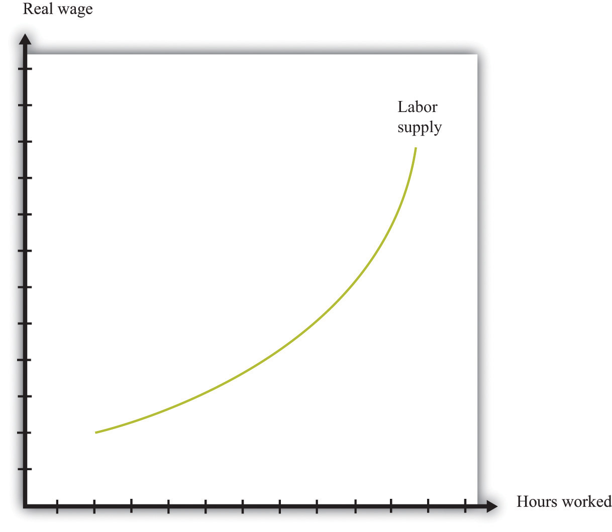
The response of the quantity of labor supplied to the real wage depends on both an income effect and a substitution effect. When the substitution effect is larger than the income effect, the supply curve has the “normal” upward-sloping shape.
In the end, the shape of the labor supply curve is an empirical question; we can answer it only by going to the data. And as you might be able to guess, it turns out to be a difficult question to answer, once we start dealing with the complexities of different kinds of labor. The view of most economists who have studied labor supply is that higher real wages do lead to a greater quantity of labor supplied, but the effect is not very strong. The income effect almost cancels out the substitution effect. This means that the labor supply curve slopes upward but is quite steep.
The Effect of the Reagan Tax Cuts on the Supply of Labor
Suppose an individual knows the nominal wage but also knows that she is going to be taxed on any income that she earns at the going income tax rate. The wage rate that matters for her decision is the after-tax real wage. Her real disposable income is
All our discussion of labor supply continues to hold in this case, except that we need to replace the real wage with the after-tax real wage since it is the after-tax wage that matters to the individual.
Figure 27.11 "Labor Supply Response to Tax Cut" shows the effect of a cut in taxes. If the labor supply curve slopes upward, the tax cut leads to an increase in the quantity of labor supplied. And if labor supply increases, then potential output also increases. In other words, one effect of tax cuts is to induce people to work harder and produce more real GDP. To keep things simple, Figure 27.11 "Labor Supply Response to Tax Cut" is drawn supposing that there is no change in the equilibrium real wage as a result of the tax cut. In fact, we would expect the real wage to decrease somewhat as well. Buyers of labor as well as sellers of labor would benefit from the tax cut. Indeed, it is this decrease in the real wage that induces firms to purchase the extra labor that individuals wish to supply. (If we included this in our picture, then the after-tax real wage would still increase but by less than shown in the figure.)
Figure 27.11 Labor Supply Response to Tax Cut
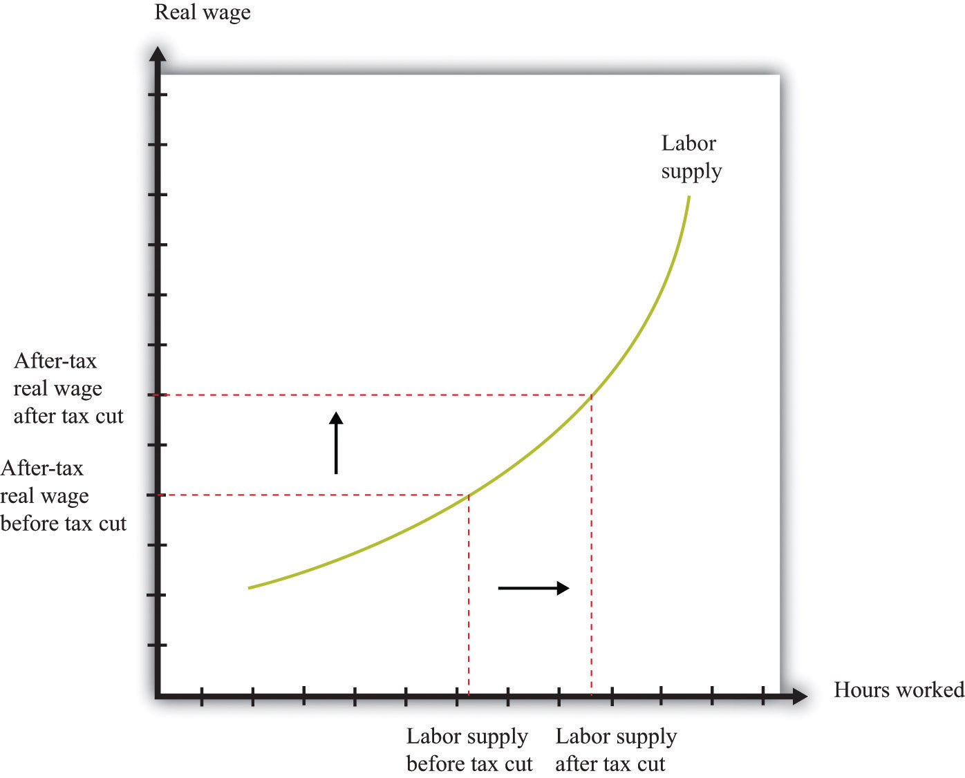
The wage that matters for labor supply decisions is the after-tax real wage. If income taxes are cut, and the real wage is unchanged, then households will supply more labor.
The Laffer Curve
Supply-side economics was controversial and generated a great deal of debate back in the 1980s and since. Yet the argument that we have just presented is not really controversial at all. Almost all economists agreed that as a matter of theory, cuts in taxes could lead to increases in the quantity of labor supplied. The disagreements concerned the magnitude of the effect.
Some proponents of supply-side economics made a much stronger claim. They said that the positive effects on labor supply could be so large that total tax revenues would increase, not decrease. They argued that even though the government would get less tax revenue on each dollar earned, people would work so much harder and generate so much more taxable income that the government would end up with more revenue than before.
This argument was encapsulated in the so-called Laffer curve. Economist Arthur Laffer asked what would happen if you graphed tax revenues as a function of the tax rate. Obviously (he observed) if the tax rate is zero, then tax revenues must be zero. And, Laffer argued, if the tax rate were 100 percent, so the government took every penny you earned, then no one would have an incentive to work at all, and the quantity of labor supplied would drop down to zero. Once again, income tax revenues would be zero. In between, tax revenues are positive.
Figure 27.12 "Laffer Curve" shows an example of a Laffer curve. There is some tax rate that will lead to the maximum possible revenue for the government. This itself is not that interesting: the goal of the government is not to raise as much tax revenue as possible. But if the tax rate lies to the right of that point, then—as the picture shows—a cut in taxes will increase tax revenues.
Figure 27.12 Laffer Curve
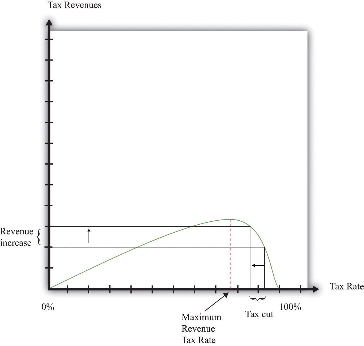
The Laffer curve says that it is possible for a reduction in the tax rate to lead to an increase in tax revenues. Although this is a theoretical possibility at very high tax rates, most economists view the Laffer curve as a theoretical curiosity with limited applicability to real economies.
Just as almost all economists agreed that there would be some supply-side effects of income tax cuts, almost all economists agreed that the Laffer curve argument was inapplicable to the US economy (or indeed any other economy). The evidence indicated that the effects of tax cuts on hours worked were likely to be relatively small. Almost no economists actually believed that the economy was on the wrong side of the Laffer curve, where tax cuts could pay for themselves.
Unfortunately, the Laffer curve argument was politically appealing, even though it was not supported by economic evidence. Buoyed by this argument, President Reagan oversaw both tax cuts and big increases in government spending. As a result, the US government ran large budget deficits. Following on from the ERTA, President Reagan and President George H. W. Bush after him were both forced to increase taxes to bring the budget back under control.The economic history of the United States in the 1980s was quite complex. Because this chapter concerns income taxes, we have considered only one of the policy changes of the Reagan administration. Other changes in tax policy were designed to promote savings. We have not discussed other aspects of President Reagan’s fiscal policy (there were large increases in government purchases), the tight monetary policy pursued by the Federal Reserve, or the behavior of interest rates and exchange rates. All these are matters for other chapters.
Key Takeaways
- Prior to the Reagan tax cut, the US economy was experiencing both low growth in real GDP and high inflation.
- Reagan’s economic advisors stressed the effects of taxes on the supply side of the economy, and in particular the incentive effects of taxes on labor supply and investment.
- The Reagan tax cuts led to considerably higher deficits in the United States.
Checking Your Understanding
- What matters for labor supply decisions—the marginal tax rate or the average tax rate?
- According to the Laffer curve, does a tax cut always increase tax revenues?