This is “Accounting for Changes in GDP”, section 20.5 from the book Theory and Applications of Economics (v. 1.0). For details on it (including licensing), click here.
For more information on the source of this book, or why it is available for free, please see the project's home page. You can browse or download additional books there. To download a .zip file containing this book to use offline, simply click here.


20.5 Accounting for Changes in GDP
Learning Objectives
After you have read this section, you should be able to answer the following questions:
- What is growth accounting?
- What are the different time horizons that we use in economics?
We have inventoried the factors that contribute to gross domestic product (GDP). The next step is to understand how much each factor contributes. If an economy wants to increase its GDP, is it better off trying to boost domestic savings, attract more capital from other countries, improve its infrastructure, or what? To answer such questions, we introduce a new tool that links the growth rateThe change in a variable over time divided by its value in the beginning period. of output to the growth rate of the different inputs to the production function.
Toolkit: Section 31.21 "Growth Rates"
A growth rate is the percentage change in a variable from one year to the next. For example, the growth rate of real GDP is defined as
You can learn more about growth rates in the toolkit.
Some of the inputs to the production function—most notably knowledge, social infrastructure, and natural resources—are very difficult to measure individually. Economists typically group these inputs together into technologyA catchall term comprising knowledge, social infrastructure, natural resources, and any other inputs to aggregate production that have not been included elsewhere., as shown in Figure 20.10 "The Aggregate Production Function". The term is something of a misnomer because it includes not only technological factors but also social infrastructure, natural resources, and indeed anything that affects real GDP but is not captured by other inputs.
Figure 20.10 The Aggregate Production Function
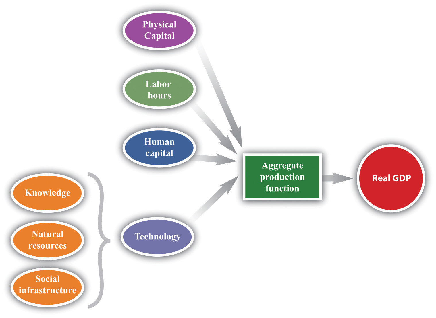
The aggregate production function combines an economy’s physical capital stock, labor hours, human capital, and technology (knowledge, natural resources, and social infrastructure) to produce output (real GDP).
The technique for explaining output growth in terms of the growth of inputs is called growth accountingAn accounting method that shows how changes in real GDP in an economy are due to changes in available inputs..
Toolkit: Section 31.28 "Growth Accounting"
Growth accounting tells us how changes in real GDP in an economy are due to changes in available inputs. Under reasonably general circumstances, the change in output in an economy can be written as follows:
output growth rate = a × capital stock growth rate + [(1 − a) × labor hours growth rate] + [(1 − a) × human capital growth rate] + technology growth rate.In this equation, a is just a number. Growth rates can be positive or negative, so we can use the equation to analyze decreases and increases in GDP.
We can measure the growth in output, capital stock, and labor hours using easily available economic data. The growth rate of human capital is trickier to measure, although we can use information on schooling and literacy rates to estimate this number. We also have a way of measuring a. The technical details are not important here, but a good measure of (1 − a) is simply total payments to labor in the economy (that is, the total of wages and other compensation) as a fraction of overall GDP. For most economies, a is in the range of about 1/3 to 1/2.
For the United States, the number a is about 1/3. The growth rate of output is therefore given as follows:
Because we can measure everything in this equation except growth in technology, we can use the equation to determine what the growth rate of technology must be. If we rearrange, we get the following:
To emphasize again, the powerful part of this equation is that we can use observed growth in labor, capital, human capital, and output to infer the growth rate of technology—something that is impossible to measure directly.
Growth Accounting in Action
Table 20.2 "Some Examples of Growth Accounting Calculations*" provides information on output growth, capital growth, labor growth, and technology growth. The calculations assume that a = 1/3. In the first row, for example, we see that
growth in technology = 5.5 − [(1/3) × 6.0] − [(2/3) × (2.0 + 1.0)] = 5.5 − 2.0 − 2.0 = 1.5.Table 20.2 Some Examples of Growth Accounting Calculations*
| Year | Output Growth | Capital Growth | Labor Growth | Human Capital Growth | Technology Growth |
|---|---|---|---|---|---|
| 2010 | 5.5 | 6.0 | 2.0 | 1.0 | 1.0 |
| 2011 | 2.0 | 3.0 | 1.5 | 0 | 0 |
| 2012 | 6.5 | 4.5 | 1.0 | 0.5 | |
| 2013 | 1.5 | 0 | 0 | 2.2 | |
| 2014 | 4.4 | 3.3 | 0 | 1.3 | |
| *The figures in each column are percentage growth rates. | |||||
Growth accounting is an extremely useful tool because it helps us diagnose the causes of economic success and failure. We can look at successful growing economies and find out if they are growing because they have more capital, labor, or skills or because they have improved their technological know-how. Likewise, we can look at economies in which output has fallen and find out whether declines in capital, labor, or technology are responsible.We use this tool in Chapter 22 "The Great Depression" to study the behavior of the US economy in the 1920s and 1930s.
Researchers have found that different countries and regions of the world have vastly varying experiences when viewed through the lens of growth accounting. A World Bank study found that, in developing regions of the world, capital accumulation was a key contributor to output growth, accounting for almost two-thirds of total growth in Africa, Latin America, East Asia, and Southeast Asia.The study covered the period 1960–1987. See World Bank, World Development Report 1991: The Challenge of Development, vol. 1, p. 45, June 30, 1991, accessed August 22, 2011, http://econ.worldbank.org/external/default/main?pagePK=64165259&theSitePK=478060&pi PK=64165421&menuPK=64166093&entityID=000009265_3981005112648. Technology and human capital growth played a surprisingly small role in these regions, contributing nothing at all to economic growth in Africa and Latin America, for example.
The Short Run, the Long Run, and the Very Long Run
Growth accounting focuses on how inputs—and hence output—change over time. We use the tool both to look at changes in an economy over short time periods—say, from one month to the next—and also over very long time periods—say, over decades. We are limited only by the data that we have available to us. It is sometimes useful to distinguish three different time horizons.
- The short run refers to a period of time that we would typically measure in months. If something has only a short-run effect on an economy, the effect will vanish within months or a few years at most.
- The long run refers to periods of time that are better measured in years. If something will happen in the long run, we might have to wait for two, three, or more years before it happens.
- The very long run refers to periods of time that are best measured in decades.
These definitions of the short, long, and very long runs are not and cannot be very exact. In the context of particular chapters, however, we give more precise definitions to these ideas.For example, Chapter 25 "Understanding the Fed" explains the adjustment of prices in an economy. In that chapter, we define the short run as the time horizon in which prices are “sticky”—not all prices have adjusted fully—whereas the long run refers to a period where all prices have fully adjusted. Meanwhile, Chapter 21 "Global Prosperity and Global Poverty" uses the very long run to refer to a situation where output and the physical capital stock grow at the same rate. Figure 20.11 "The Different Time Horizons in Economics" summarizes the main influences on the inputs to the production function in the short run, the long run, and the very long run.
Figure 20.11 The Different Time Horizons in Economics
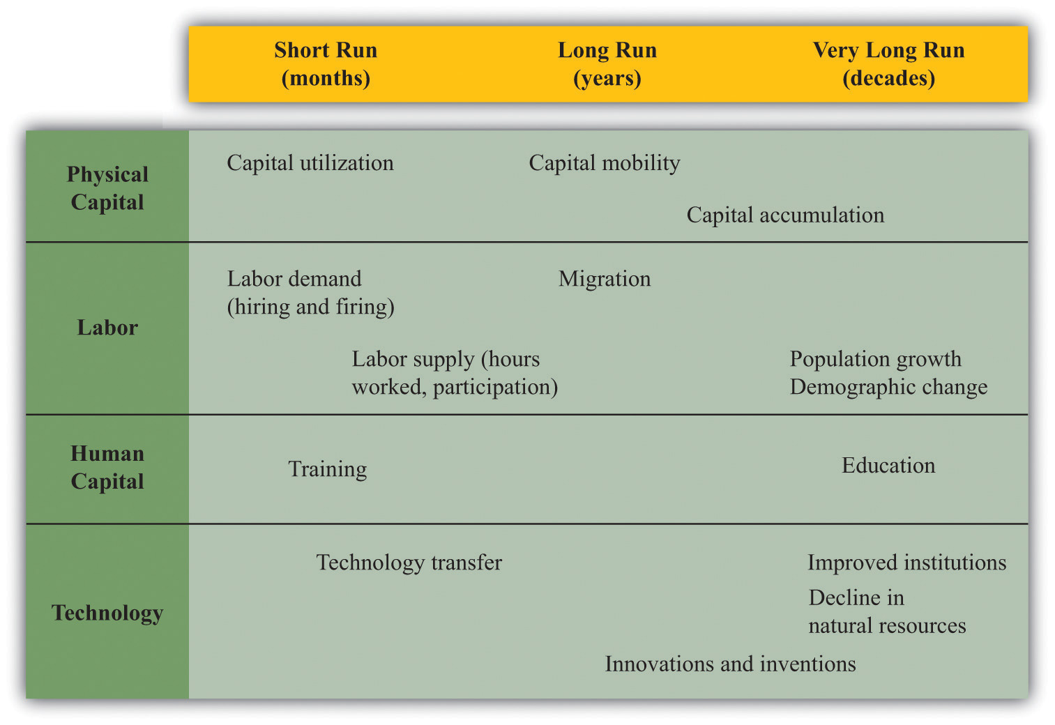
Look first at physical capital—the first row in Figure 20.11 "The Different Time Horizons in Economics". In the short run, the amount of physical capital in the economy is more or less fixed. There are a certain number of machines, buildings, and so on, and we cannot make big changes in this capital stock. One thing that firms can do in the short run is to change capital utilization—shutting down a production line if they want to produce less output or running extra shifts if they want more output. Once we move to the long run and very long run, capital mobility and capital accumulation become important.
Look next at labor. In the short run, the amount of labor in the production function depends primarily on how much labor firms want to hire (labor demand) and how much people want to work (labor supply). As we move to the long run, migration of labor becomes significant as well: workers sometimes move from one country to another in search of better jobs. And, in the very long run, population growth and other demographic changes (the aging of the population, the increased entry of women into the labor force, etc.) start to matter.
Human capital can be increased in the long run (and also in the short run to some extent) by training. The most important changes in human capital come in the very long run, however, through improved education.
There is not very much that can be done to change a country’s technology in the short run. In the long run, less technologically advanced countries can import better technologies from other countries. In practice, this often happens as a result of a multinational firm establishing operations in a developing country. For example, if Dell Inc. establishes a factory in Mexico, then it effectively transfers some know-how to the Mexican economy. This is known as technology transferThe movement of knowledge and advanced production techniques across national borders., the movement of knowledge and advanced production techniques across national borders.
In the long run and very long run, technology advances through innovation and the hard work of research and development (R&D) that—hopefully—gives us new inventions. In the very long run, countries may be able to improve their institutions and thus create better social infrastructure. In the very long run, declines in natural resources also become significant.
Key Takeaways
- Growth accounting is a tool to decompose economic growth into components of input growth and technological progress.
- In economics, we study changes in GDP over very different time horizons. We look at short-run changes due mainly to changes in hours worked and the utilization of capital stock. We look at long-run changes due to changes in the amount of available labor and capital in an economy. And we look at very-long-run changes due to the accumulation of physical and human capital and changes in social infrastructure and other aspects of technology.
Checking Your Understanding
- Rewrite the growth accounting equation for the case where a = 1/4.
- Using the growth accounting equation, fill in the missing numbers in Table 20.2 "Some Examples of Growth Accounting Calculations*".