This is “The Production Possibility Frontier (Variable Proportions)”, section 5.8 from the book Policy and Theory of International Trade (v. 1.0). For details on it (including licensing), click here.
For more information on the source of this book, or why it is available for free, please see the project's home page. You can browse or download additional books there. To download a .zip file containing this book to use offline, simply click here.


5.8 The Production Possibility Frontier (Variable Proportions)
Learning Objective
- Learn how the shift from a fixed proportions to a variable proportions model affects the presentation of the Heckscher-Ohlin (H-O) model.
The production possibility frontier can be derived in the case of variable proportions by using the same labor and capital constraints used in the case of fixed proportions, but with one important adjustment. Under variable proportions, the unit factor requirements are functions of the wage-rental ratio (w/r). This implies that the capital-labor ratios (which are the ratios of the unit factor requirements) in each industry are also functions of the wage-rental ratio. If there is a change in the equilibrium (for some reason) such that the wage-rental rate rises, then labor will become relatively more expensive compared to capital. Firms would respond to this change by reducing their demand for labor and raising their demand for capital. In other words, firms will substitute capital for labor and the capital-labor ratio will rise in each industry. This adjustment will allow the firm to maintain minimum production costs and thus the highest profit possible. This is the first important distinction between variable and fixed proportions.
The second important distinction is that variable proportions change the shape of the economy’s PPF. The labor constraint with full employment can be written as
where aLC and aLW are functions of (w/r).
The capital constraint with full employment becomes
where aKC and aKW are functions of (w/r).
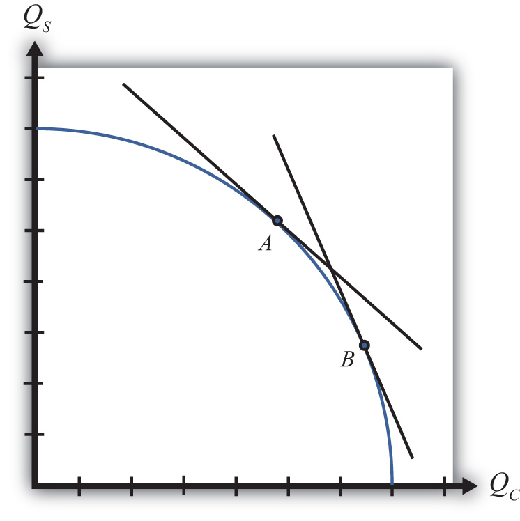
Under variable proportions, the production possibility frontier takes the traditional bowed-out shape, as shown in Figure 5.6 "The PPF in the Variable Proportions H-O Model". All points on the PPF will maintain full employment of both labor and capital resources. The slope of a line tangent to the PPF (such as the line through point A) represents the quantity of steel that must be given up to produce another unit of clothing. As such, the slope of the PPF is the opportunity cost of producing clothing. Since the slope becomes steeper as more and more clothing is produced (as when moving production from point A to B), we say that there is increasing opportunity cost. This means that more steel must be given up to produce one more unit of clothing at point B than at point A in the figure. In contrast, in the Ricardian model the PPF was a straight line that indicated constant opportunity costs.
Figure 5.6 The PPF in the Variable Proportions H-O Model
The third important distinction of variable proportions is that the magnification effects, derived previously under a fixed proportions assumption, continue to work under variable proportions. To show this requires a fair amount of advanced math, but a student can rest assured that we can apply the magnification effect even in the more complex variable proportions version of the Heckscher-Ohlin (H-O) model.
Key Takeaways
- Variable proportions imply that the capital-labor ratios used in production are varied as wage and rental rates change in the economy.
- Variable proportions imply that the PPF becomes bowed out and continuous, consisting of many output combinations that can be produced with full employment of labor and capital.
- Variable proportions do not invalidate the Rybczynski theorem, the Stolper-Samuelson theorem, or the magnification effects for quantities and prices.
Exercise
-
Jeopardy Questions. As in the popular television game show, you are given an answer to a question and you must respond with the question. For example, if the answer is “a tax on imports,” then the correct question is “What is a tariff?”
- Interpretation given for the slope of the production possibility frontier in the case of variable proportions in the Heckscher-Ohlin model.
- In a variable proportion H-O model, the factor proportions in each industry vary with changes in these two other variables.
- Of increase, decrease, or stay the same, this is the effect on the capital-labor ratio in an industry when wages fall in a variable proportions H-O model.
- Of increase, decrease, or stay the same, this is the effect on the amount of capital used per worker in an industry when rental rates increase in a variable proportions H-O model.
- Of increase, decrease, or stay the same, this is the effect on the labor-capital ratio in an industry when wages fall in a variable proportions H-O model.
- Of increase, decrease, or stay the same, this is the effect on the capital-labor ratio in the cheese industry when wages increase in a variable proportions H-O model, if cheese is a labor-intensive industry.
- Of increase, decrease, or stay the same, this is the effect on the capital-labor ratio in the wine industry when wages increase in a variable proportions H-O model, if wine is a capital-intensive industry.
- Of increase, decrease, or stay the same, this is the effect on the capital-labor ratio in an industry when wages fall in a fixed proportions H-O model.