This is “Vector Data Models”, section 4.2 from the book Geographic Information System Basics (v. 1.0). For details on it (including licensing), click here.
For more information on the source of this book, or why it is available for free, please see the project's home page. You can browse or download additional books there. To download a .zip file containing this book to use offline, simply click here.


4.2 Vector Data Models
Learning Objective
- The objective of this section is to understand how vector data models are implemented in GIS applications.
In contrast to the raster data model is the vector data model. In this model, space is not quantized into discrete grid cells like the raster model. Vector data models use points and their associated X, Y coordinate pairs to represent the vertices of spatial features, much as if they were being drawn on a map by hand (Aronoff 1989).Aronoff, S. 1989. Geographic Information Systems: A Management Perspective. Ottawa, Canada: WDL Publications. The data attributes of these features are then stored in a separate database management system. The spatial information and the attribute information for these models are linked via a simple identification number that is given to each feature in a map.
Three fundamental vector types exist in geographic information systems (GISs): points, lines, and polygons (Figure 4.8 "Points, Lines, and Polygons"). PointsA zero-dimensional object containing a single coordinate pair. In a GIS, points have only the property of location. are zero-dimensional objects that contain only a single coordinate pair. Points are typically used to model singular, discrete features such as buildings, wells, power poles, sample locations, and so forth. Points have only the property of location. Other types of point features include the nodeThe intersection points where two or more arcs meet. and the vertexA corner or a point where lines meet.. Specifically, a point is a stand-alone feature, while a node is a topological junction representing a common X, Y coordinate pair between intersecting lines and/or polygons. Vertices are defined as each bend along a line or polygon feature that is not the intersection of lines or polygons.
Figure 4.8 Points, Lines, and Polygons
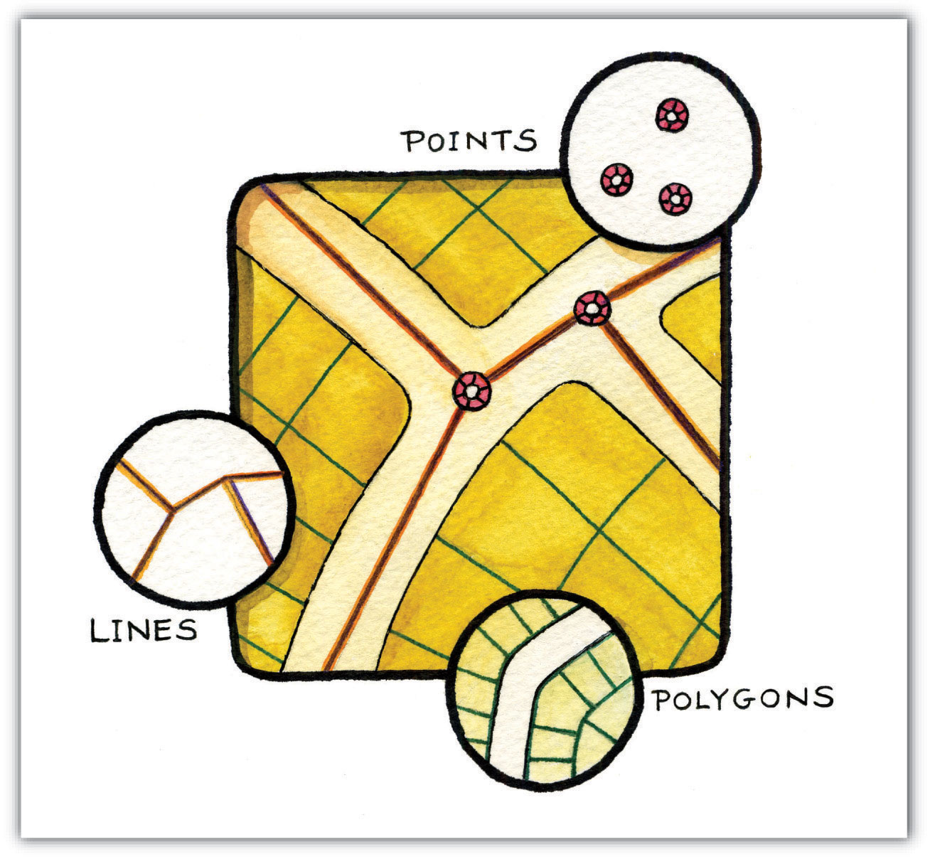
Points can be spatially linked to form more complex features. LinesA one-dimensional object composed of multiple, explicitly connected points. Lines have the property of length. Also called an “arc.” are one-dimensional features composed of multiple, explicitly connected points. Lines are used to represent linear features such as roads, streams, faults, boundaries, and so forth. Lines have the property of length. Lines that directly connect two nodes are sometimes referred to as chains, edges, segments, or arcsA one-dimensional object composed of multiple, explicitly connected points. Lines have the property of length. Also called a “line.”.
PolygonsA two-dimensional feature created from multiple lines that loop back to create a “closed” feature. Polygons have the properties of area and perimeter. Also called “areas.” are two-dimensional features created by multiple lines that loop back to create a “closed” feature. In the case of polygons, the first coordinate pair (point) on the first line segment is the same as the last coordinate pair on the last line segment. Polygons are used to represent features such as city boundaries, geologic formations, lakes, soil associations, vegetation communities, and so forth. Polygons have the properties of area and perimeter. Polygons are also called areasA two-dimensional feature created from multiple lines that loop back to create a “closed” feature. Areas have the properties of area and perimeter. Also called “polygons.”.
Vector Data Models Structures
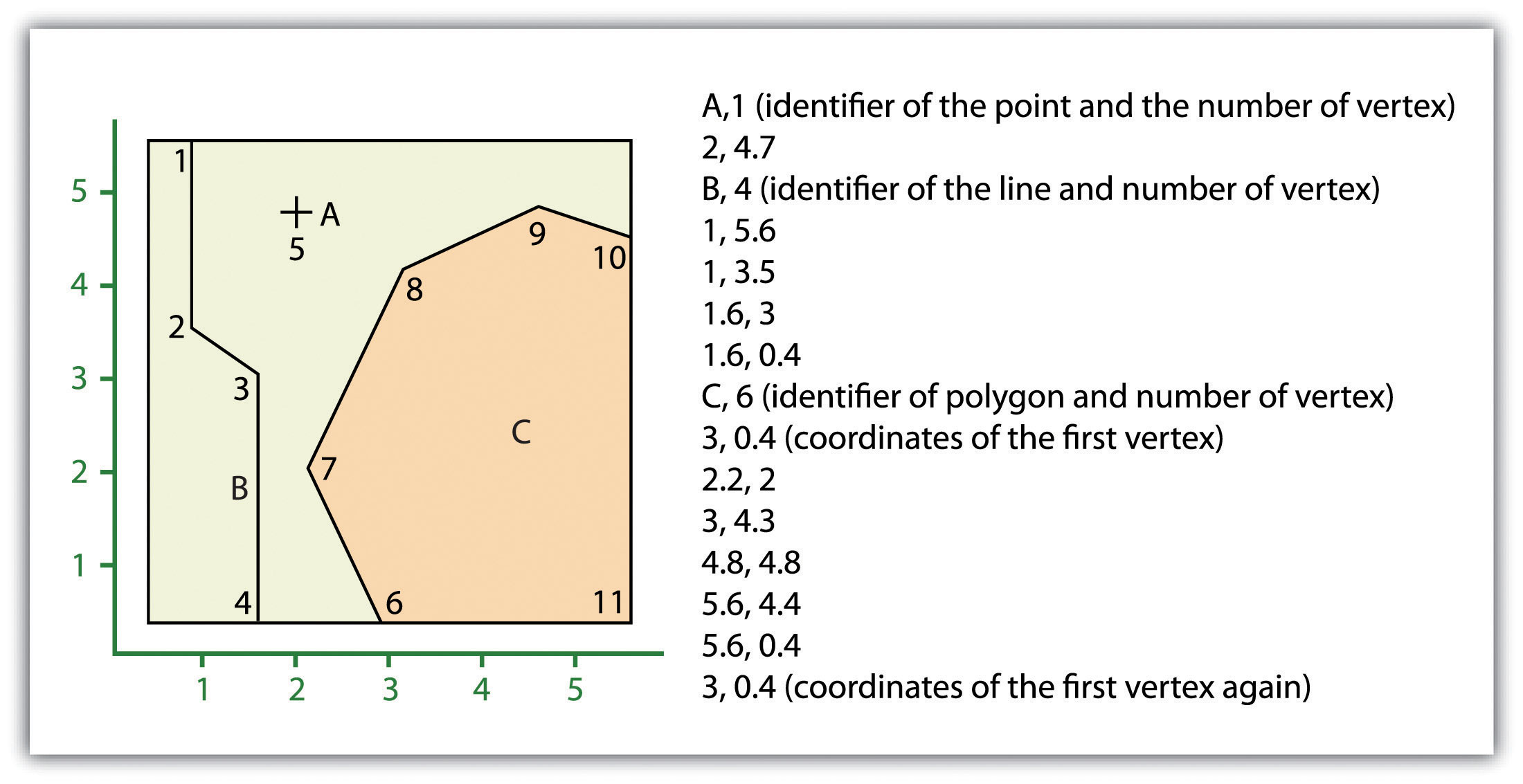
Vector data models can be structured many different ways. We will examine two of the more common data structures here. The simplest vector data structure is called the spaghetti data modelA data model in which each point, line, and/or polygon feature is represented as a string of X, Y coordinate pairs with no inherent structure. (Dangermond 1982).Dangermond, J. 1982. “A Classification of Software Components Commonly Used in Geographic Information Systems.” In Proceedings of the U.S.-Australia Workshop on the Design and Implementation of Computer-Based Geographic Information Systems, 70–91. Honolulu, HI. In the spaghetti model, each point, line, and/or polygon feature is represented as a string of X, Y coordinate pairs (or as a single X, Y coordinate pair in the case of a vector image with a single point) with no inherent structure (Figure 4.9 "Spaghetti Data Model"). One could envision each line in this model to be a single strand of spaghetti that is formed into complex shapes by the addition of more and more strands of spaghetti. It is notable that in this model, any polygons that lie adjacent to each other must be made up of their own lines, or stands of spaghetti. In other words, each polygon must be uniquely defined by its own set of X, Y coordinate pairs, even if the adjacent polygons share the exact same boundary information. This creates some redundancies within the data model and therefore reduces efficiency.
Figure 4.9 Spaghetti Data Model
Despite the location designations associated with each line, or strand of spaghetti, spatial relationships are not explicitly encoded within the spaghetti model; rather, they are implied by their location. This results in a lack of topological information, which is problematic if the user attempts to make measurements or analysis. The computational requirements, therefore, are very steep if any advanced analytical techniques are employed on vector files structured thusly. Nevertheless, the simple structure of the spaghetti data model allows for efficient reproduction of maps and graphics as this topological information is unnecessary for plotting and printing.
In contrast to the spaghetti data model, the topological data modelA data model characterized by the inclusion of topology. is characterized by the inclusion of topological information within the dataset, as the name implies. TopologyA set of rules that models the relationship between neighboring points, lines, and polygons and determines how they share geometry. Topology is also concerned with preserving spatial properties when the forms are bent, stretched, or placed under similar geometric transformation. is a set of rules that model the relationships between neighboring points, lines, and polygons and determines how they share geometry. For example, consider two adjacent polygons. In the spaghetti model, the shared boundary of two neighboring polygons is defined as two separate, identical lines. The inclusion of topology into the data model allows for a single line to represent this shared boundary with an explicit reference to denote which side of the line belongs with which polygon. Topology is also concerned with preserving spatial properties when the forms are bent, stretched, or placed under similar geometric transformations, which allows for more efficient projection and reprojection of map files.
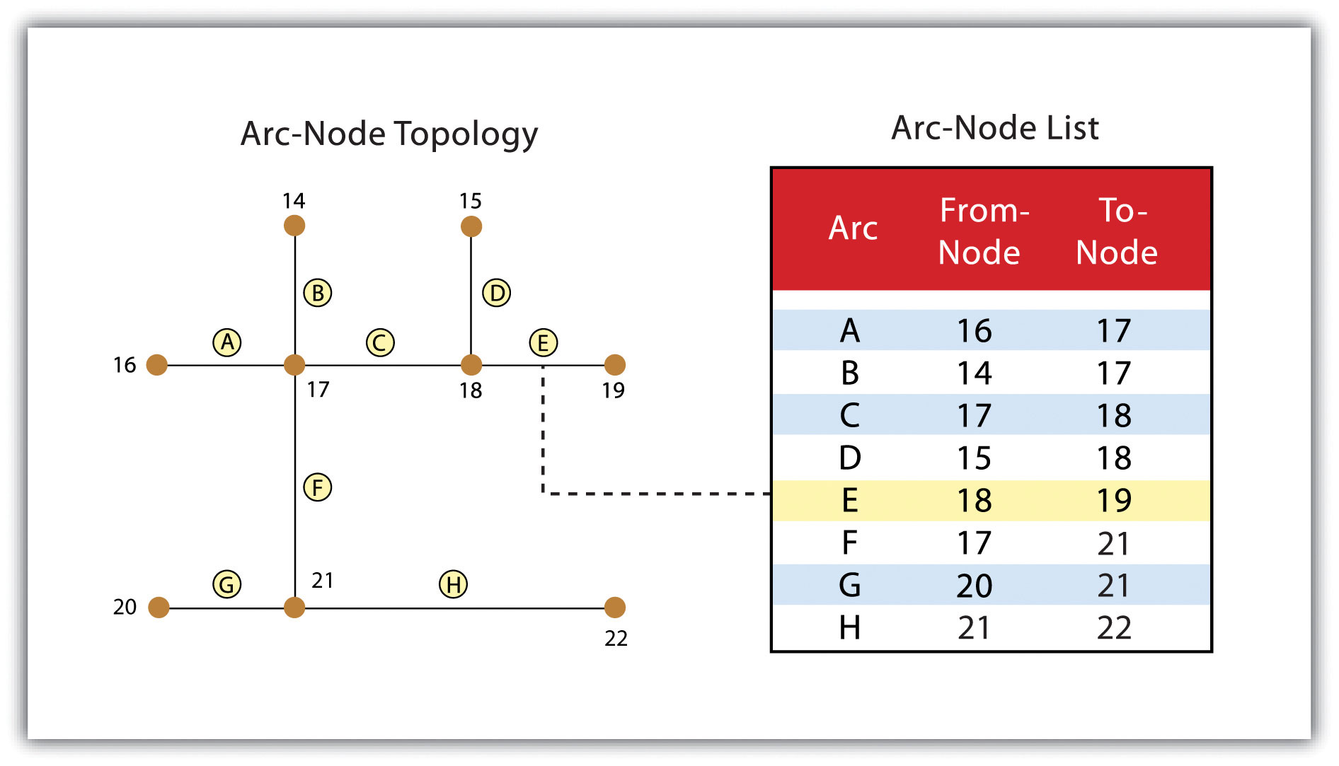
Three basic topological precepts that are necessary to understand the topological data model are outlined here. First, connectivityThe topological property of lines sharing a common node. describes the arc-node topology for the feature dataset. As discussed previously, nodes are more than simple points. In the topological data model, nodes are the intersection points where two or more arcs meet. In the case of arc-node topology, arcs have both a from-node (i.e., starting node) indicating where the arc begins and a to-node (i.e., ending node) indicating where the arc ends (Figure 4.10 "Arc-Node Topology"). In addition, between each node pair is a line segment, sometimes called a link, which has its own identification number and references both its from-node and to-node. In Figure 4.10 "Arc-Node Topology", arcs 1, 2, and 3 all intersect because they share node 11. Therefore, the computer can determine that it is possible to move along arc 1 and turn onto arc 3, while it is not possible to move from arc 1 to arc 5, as they do not share a common node.
Figure 4.10 Arc-Node Topology
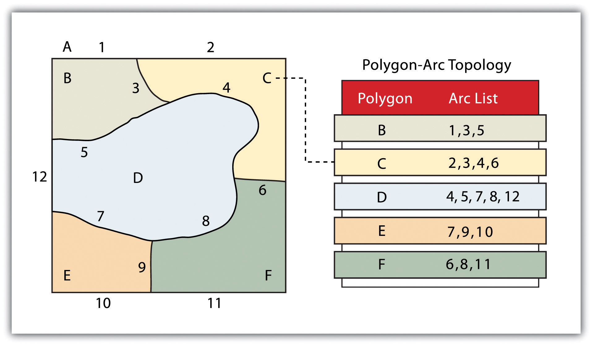
The second basic topological precept is area definitionThe topological property stating that line segments connect to surround an area and define a polygon.. Area definition states that an arc that connects to surround an area defines a polygon, also called polygon-arc topology. In the case of polygon-arc topology, arcs are used to construct polygons, and each arc is stored only once (Figure 4.11 "Polygon-Arc Topology"). This results in a reduction in the amount of data stored and ensures that adjacent polygon boundaries do not overlap. In the Figure 4.11 "Polygon-Arc Topology", the polygon-arc topology makes it clear that polygon F is made up of arcs 8, 9, and 10.
Figure 4.11 Polygon-Arc Topology
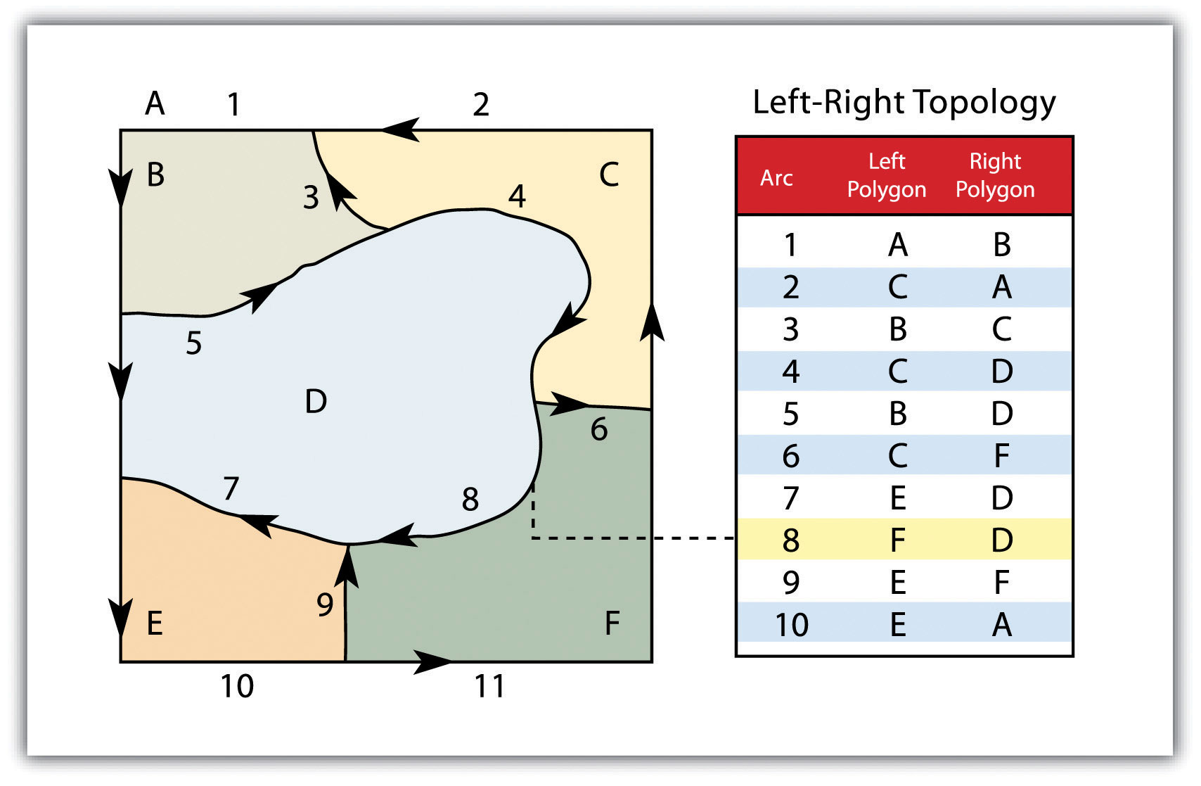
ContiguityThe topological property of identifying adjacent polygons by recording the left and right side of each line segment., the third topological precept, is based on the concept that polygons that share a boundary are deemed adjacent. Specifically, polygon topology requires that all arcs in a polygon have a direction (a from-node and a to-node), which allows adjacency information to be determined (Figure 4.12 "Polygon Topology"). Polygons that share an arc are deemed adjacent, or contiguous, and therefore the “left” and “right” side of each arc can be defined. This left and right polygon information is stored explicitly within the attribute information of the topological data model. The “universe polygon” is an essential component of polygon topology that represents the external area located outside of the study area. Figure 4.12 "Polygon Topology" shows that arc 6 is bound on the left by polygon B and to the right by polygon C. Polygon A, the universe polygon, is to the left of arcs 1, 2, and 3.
Figure 4.12 Polygon Topology
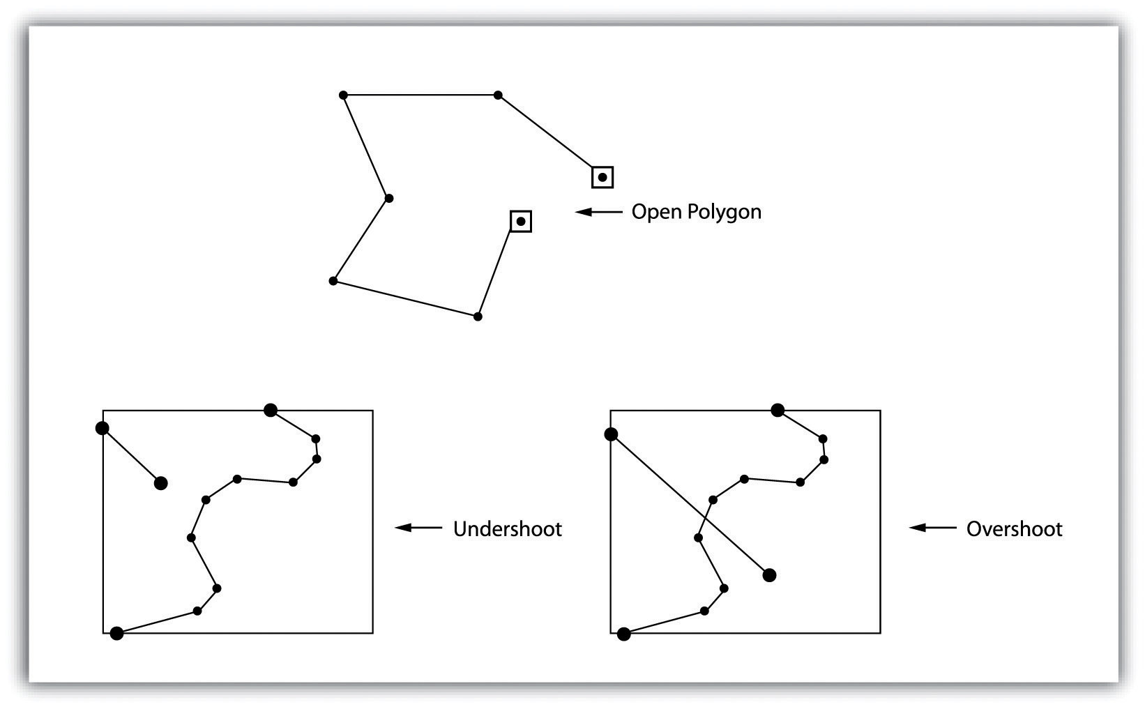
Topology allows the computer to rapidly determine and analyze the spatial relationships of all its included features. In addition, topological information is important because it allows for efficient error detection within a vector dataset. In the case of polygon features, open or unclosed polygons, which occur when an arc does not completely loop back upon itself, and unlabeled polygons, which occur when an area does not contain any attribute information, violate polygon-arc topology rules. Another topological error found with polygon features is the sliverA narrow gap formed when the shared boundary of two polygons do not meet exactly.. Slivers occur when the shared boundary of two polygons do not meet exactly (Figure 4.13 "Common Topological Errors").
In the case of line features, topological errors occur when two lines do not meet perfectly at a node. This error is called an “undershoot” when the lines do not extend far enough to meet each other and an “overshoot” when the line extends beyond the feature it should connect to (Figure 4.13 "Common Topological Errors"). The result of overshoots and undershoots is a “dangling node” at the end of the line. Dangling nodes aren’t always an error, however, as they occur in the case of dead-end streets on a road map.
Figure 4.13 Common Topological Errors
Many types of spatial analysis require the degree of organization offered by topologically explicit data models. In particular, network analysis (e.g., finding the best route from one location to another) and measurement (e.g., finding the length of a river segment) relies heavily on the concept of to- and from-nodes and uses this information, along with attribute information, to calculate distances, shortest routes, quickest routes, and so forth. Topology also allows for sophisticated neighborhood analysis such as determining adjacency, clustering, nearest neighbors, and so forth.
Now that the basics of the concepts of topology have been outlined, we can begin to better understand the topological data model. In this model, the node acts as more than just a simple point along a line or polygon. The node represents the point of intersection for two or more arcs. Arcs may or may not be looped into polygons. Regardless, all nodes, arcs, and polygons are individually numbered. This numbering allows for quick and easy reference within the data model.
Advantages/Disadvantages of the Vector Model
In comparison with the raster data model, vector data models tend to be better representations of reality due to the accuracy and precision of points, lines, and polygons over the regularly spaced grid cells of the raster model. This results in vector data tending to be more aesthetically pleasing than raster data.
Vector data also provides an increased ability to alter the scale of observation and analysis. As each coordinate pair associated with a point, line, and polygon represents an infinitesimally exact location (albeit limited by the number of significant digits and/or data acquisition methodologies), zooming deep into a vector image does not change the view of a vector graphic in the way that it does a raster graphic (see Figure 4.1 "Digital Picture with Zoomed Inset Showing Pixilation of Raster Image").
Vector data tend to be more compact in data structure, so file sizes are typically much smaller than their raster counterparts. Although the ability of modern computers has minimized the importance of maintaining small file sizes, vector data often require a fraction the computer storage space when compared to raster data.
The final advantage of vector data is that topology is inherent in the vector model. This topological information results in simplified spatial analysis (e.g., error detection, network analysis, proximity analysis, and spatial transformation) when using a vector model.
Alternatively, there are two primary disadvantages of the vector data model. First, the data structure tends to be much more complex than the simple raster data model. As the location of each vertex must be stored explicitly in the model, there are no shortcuts for storing data like there are for raster models (e.g., the run-length and quad-tree encoding methodologies).
Second, the implementation of spatial analysis can also be relatively complicated due to minor differences in accuracy and precision between the input datasets. Similarly, the algorithms for manipulating and analyzing vector data are complex and can lead to intensive processing requirements, particularly when dealing with large datasets.
Key Takeaways
- Vector data utilizes points, lines, and polygons to represent the spatial features in a map.
- Topology is an informative geospatial property that describes the connectivity, area definition, and contiguity of interrelated points, lines, and polygon.
- Vector data may or may not be topologically explicit, depending on the file’s data structure.
- Care should be taken to determine whether the raster or vector data model is best suited for your data and/or analytical needs.
Exercises
- What vector type (point, line, or polygon) best represents the following features: state boundaries, telephone poles, buildings, cities, stream networks, mountain peaks, soil types, flight tracks? Which of these features can be represented by multiple vector types? What conditions might lead you choose one vector type over another?
- Draw a point, line, and polygon feature on a simple Cartesian coordinate system. From this drawing, create a spaghetti data model that approximates the shapes shown therein.
- Draw three adjacent polygons on a simple Cartesian coordinate system. From this drawing, create a topological data model that incorporates arc-node, polygon-arc, and polygon topology.