This is “Aggregate Demand Curve”, section 22.3 from the book Finance, Banking, and Money (v. 2.0). For details on it (including licensing), click here.
For more information on the source of this book, or why it is available for free, please see the project's home page. You can browse or download additional books there. To download a .zip file containing this book to use offline, simply click here.
22.3 Aggregate Demand Curve
Learning Objective
- What is the aggregate demand (AD) curve and what causes it to shift?
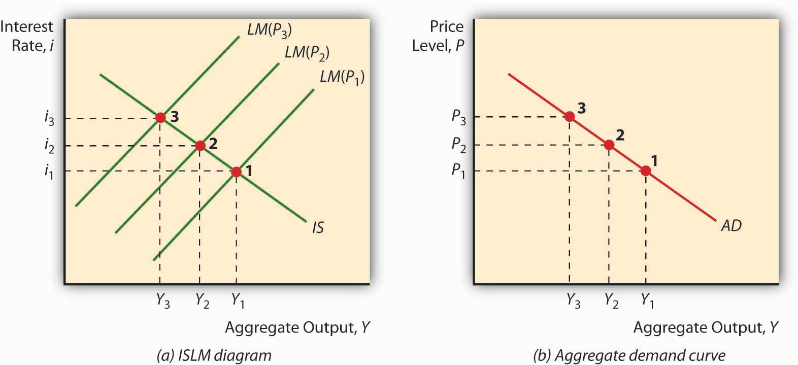
Imagine a fixed IS curve and an LM curve shifting hard left due to increases in the price level, as in Figure 22.6 "Deriving the aggregate demand curve". As prices increase, Y falls and i rises. Now plot that outcome on a new graph, where aggregate output Y remains on the horizontal axis but the vertical axis is replaced by the price level P. The resulting curve, called the aggregate demand (AD) curve, will slope downward, as below. The AD curve is a very powerful tool because it indicates the points at which equilibrium is achieved in the markets for goods and money at a given price level. It slopes downward because a high price level, ceteris paribus, means a small real money supply, high interest rates, and a low level of output, while a low price level, all else constant, is consistent with a larger real money supply, low interest rates, and kickin’ output.
Figure 22.6 Deriving the aggregate demand curve

Because the AD curve is essentially just another way of stating the IS-LM model, anything that would change the IS or LM curves will also shift the AD curve. More specifically, the AD curve shifts in the same direction as the IS curve, so it shifts right (left) with autonomous increases (decreases) in C, I, G, and NX and decreases (increases) in T. The AD curve also shifts in the same direction as the LM curve. So if MS increases (decreases), it shifts right (left), and if Md increases (decreases) it shifts left (right), as in Figure 22.3 "Predicted effects of changes in major macroeconomic variables".
Key Takeaways
- The aggregate demand curve is a downward sloping curve plotted on a graph with Y on the horizontal axis and the price level on the vertical axis.
- The AD curve represents IS-LM equilibrium points, that is, equilibrium in the market for both goods and money.
- It slopes downward because, as the price level increases, the LM curve shifts left as real money balances fall.
- AD shifts in the same direction as the IS or LM curves, so anything that shifts those curves shifts AD in precisely the same direction and for the same reasons.


