16.1 The Federal Funds Market and Reserves

Central banks have three primary tools for influencing the money supply: the reserve requirement, discount loans, and open market operations. The first, as we saw in Chapter 14 "The Money Supply Process" and Chapter 15 "The Money Supply and the Money Multiplier", works through the money multiplier, constraining multiple deposit expansion the larger it becomes. Central banks today rarely use it because most banks work around reserve requirements. The second and third tools influence the monetary base (MB = C + R). Discount loans depend on banks (or nonbank borrowers, where applicable) first borrowing from, then repaying loans to, the central bank, which therefore does not have precise control over MB. Open market operations (OMO) are generally preferred as a policy tool because the central bank can easily expand or contract MB to a precise level. Using OMO, central banks can also reverse mistakes quickly.

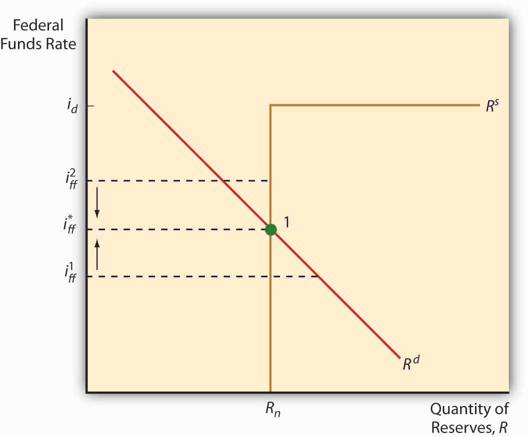
In the United States, under typical conditions, the Fed conducts monetary policy primarily through the federal funds (fed funds) market, an overnight market where banks that need reserves can borrow them from banks that hold reserves they don’t need. Banks can also borrow their reserves directly from the Fed, but, except during crises, most prefer not to because the Fed’s discount rate is generally higher than the federal funds rate. Also, borrowing too much, too often from the Fed can induce increased regulatory scrutiny. So usually banks get their overnight funds from the fed funds market, which, as Figure 16.1 "Equilibrium in the fed funds market" shows, pretty much works like any other market.

Figure 16.1 Equilibrium in the fed funds market

The downward slope of the demand curve for reserves is easily explained. Like anything else, as the price of reserves (in this case, the interest rate paid for them) increases, the quantity demanded decreases. As reserves get cheaper, banks will want more of them because the opportunity cost of that added protection, of that added liquidity, is lower. But what is the deal with that upside down L-looking reserve supply curve? Note that the curve takes a hard right (becomes infinitely elastic) at the discount rate. That’s because, if the federal funds rate ever exceeded the discount rate, banks’ thirst for Fed discount loans would be unquenchable because a clear arbitrage opportunity would exist: borrow at the discount rate and relend at the higher market rate. Below that point, the reserve supply curve is vertical (perfectly inelastic) at whatever quantity the Fed wants to supply via open market operations.

The intersection of the supply and demand curves is the equilibrium or market rate, the actual federal funds rate, ff*. When the Fed makes open market purchases, the supply of reserves shifts right, lowering ff* (ceteris paribus). When it sells, it moves the reserve supply curve left, increasing ff*, all else constant. The discount rate sets an upper limit to ff* because no bank would borrow reserves at a higher rate in the federal funds market than it could borrow directly from the Fed.

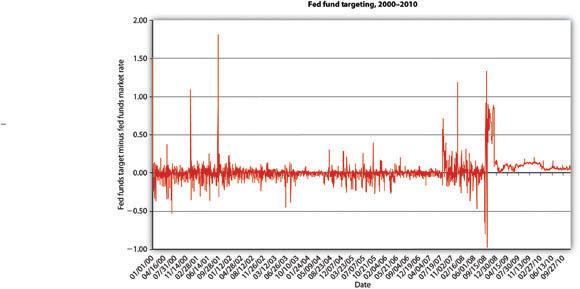
Figure 16.2 Fed funds targeting, 2000–2010

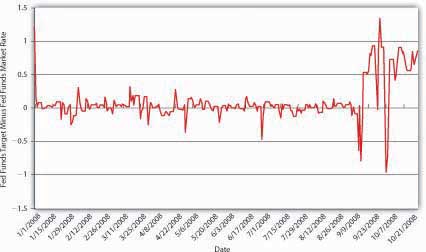
Figure 16.3 Fed funds targeting, 2008

Theoretically, the Fed could also directly affect the demand for reserves by changing the reserve requirement. If it increased (decreased) rr, demand for reserves would shift up (down), increasing (decreasing) ff*. As noted above, however, banks these days can so easily sidestep required reserves that the Fed’s ability to influence the demand for reserves is extremely limited. Demand for reserves can also shift right or left due to bank liquidity management activities, increasing (decreasing) as expectations of net deposit outflows increase (decrease). The Fed tries to anticipate such shifts and generally has done a good job of it. Although there have been days when ff* differed from the target by several percentage points (several hundred basis points), between 1982 and 2007, the fed funds target was, on average, only .0340 of a percent lower than ff*. Between 2000 and the subprime mortgage uproar in the summer of 2007, the Fed did an even better job of moving ff* to its target, as Figure 16.2 "Fed funds targeting, 2000–2010" shows. During the crises of 2007 and 2008, however, the Fed often missed its target by a long way, as shown in Figure 16.3 "Fed funds targeting, 2008". So in December 2008 it stopped publishing a feds fund target and instead began to publish the upper limit it was willing to tolerate.