This is “Inflation and Money”, chapter 25 from the book Finance, Banking, and Money (v. 1.0). For details on it (including licensing), click here.
For more information on the source of this book, or why it is available for free, please see the project's home page. You can browse or download additional books there. To download a .zip file containing this book to use offline, simply click here.


Chapter 25 Inflation and Money
Chapter Objectives
By the end of this chapter, students should be able to:
- Describe the strongest evidence for the reduced-form model that links money supply growth to inflation.
- Explain what the aggregate supply-aggregate demand (AS-AD) model, a structural model, says about money supply growth and the price level.
- Explain why central bankers allow inflation to occur year after year.
- Define lags and explain their importance.
25.1 Empirical Evidence of a Money-Inflation Link
Learning Objectives
- What is the strongest evidence for the reduced-form model that links money supply growth to inflation?
- What does the AS-AD model, a structural model, say about money supply growth and the price level?
Milton Friedman claimed that “inflation is always and everywhere a monetary phenomenon.”A Monetary History of the United States, 1867–1960. We know this isn’t entirely true because, as we saw in Chapter 23 "Aggregate Supply and Demand, the Growth Diamond, and Financial Shocks", negative aggregate supply shocks and increases in aggregate demand due to fiscal stimulus can also cause the price level to increase. Large, sustained increases in the price level, however, are indeed caused by increases in the money supply and only by increases in the money supply. The evidence for this is overwhelming: all periods of hyperinflation from the American and French Revolutions to the German hyperinflation following World War I, to more recent episodes in Latin America and Zimbabwe, have been accompanied by high rates of money supply (MS) growth. Moreover, the MS increases in some circumstances were exogenous, so those episodes were natural experiments that give us confidence that the reduced-form model correctly considers money supply as the causal agent and that reverse causation or omitted variables are unlikely.
Stop and Think Box
During the American Civil War, the Confederate States of America (CSA, or the South) issued more than $1 billion of fiat paper currency similar to today’s Federal Reserve notes, far more than the economy could support at the prewar price level. Confederate dollars fell in value from 82.7 cents in specie in 1862 to 29.0 cents in 1863, to 1.7 cents in 1865, a level of currency depreciation (inflation) that some economists think was simply too high to be accounted for by Confederate money supply growth alone. What other factors may have been at play? (Hint: Over the course of the war, the Union [the North] imposed a blockade of southern trade that increased in efficiency during the course of the war, especially as major Confederate seaports like New Orleans and Norfolk fell under northern control.)
A negative supply shock, the almost complete cutoff of foreign trade, could well have hit poor Johnny Reb (the South) as well. That would have decreased output and driven prices higher, prices already raised to lofty heights by continual emissions of too much money.
Economists also have a structural model showing a causal link between money supply growth and inflation at their disposal, the AS-AD model. Recall that an increase in MS causes the AD curve to shift right. That, in turn, causes the short-term AS curve to shift left, leading to a return to Ynrl but higher prices. If the MS grows and grows, prices will go up and up, as in Figure 25.1 "Inflation as a response to a continually increasing money supply".
Figure 25.1 Inflation as a response to a continually increasing money supply
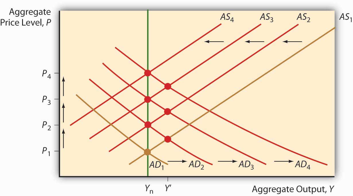
Nothing else, it turns out, can keep prices rising, rising, ever rising like that because other variables are bounded. An increase in government expenditure G will also cause AD to shift right and AS to shift left, leaving the economy with the same output but higher prices in the long run (whatever that is). But if G stops growing, as it must, then P* stops rising and inflation (the change in P*) goes to zero. Ditto with tax cuts, which can’t fall below zero (or even get close to it). So fiscal policy alone can’t create a sustained rise in prices. (Or a sustained decrease either.)
Negative supply shocks are also one-off events, not the stuff of sustained increases in prices. An oil embargo or a wage push will cause the price level to increase (and output to fall, ouch!) and negative shocks may even follow each other in rapid succession. But once the AS curve is done shifting, that’s it—P* stays put. Moreover, if Y* falls below Ynrl, in the long run (again, whatever that is), increased unemployment and other slack in the economy will cause AS to shift back to the right, restoring both output and the former price level!
So, again, Friedman was right: inflation, in the sense of continual increases in prices, is always a monetary phenomenon and only a monetary phenomenon.This is not to say, however, that negative demand shocks might not contribute to a general monetary inflation.
Stop and Think Box
Figure 25.2 "U.S. M1 and P growth" compares inflation with M1 growth laggedThe time it takes for a policy to change on a variable, a cause to create an observable effect. two years. What does the data tell you? Now look at Figure 25.3 "Government debt-to-GDP ratio" and Figure 25.4 "U.S. unemployment rates, 1961–1972". What caused M1 to grow during the 1960s?
Figure 25.2 U.S. M1 and P growth
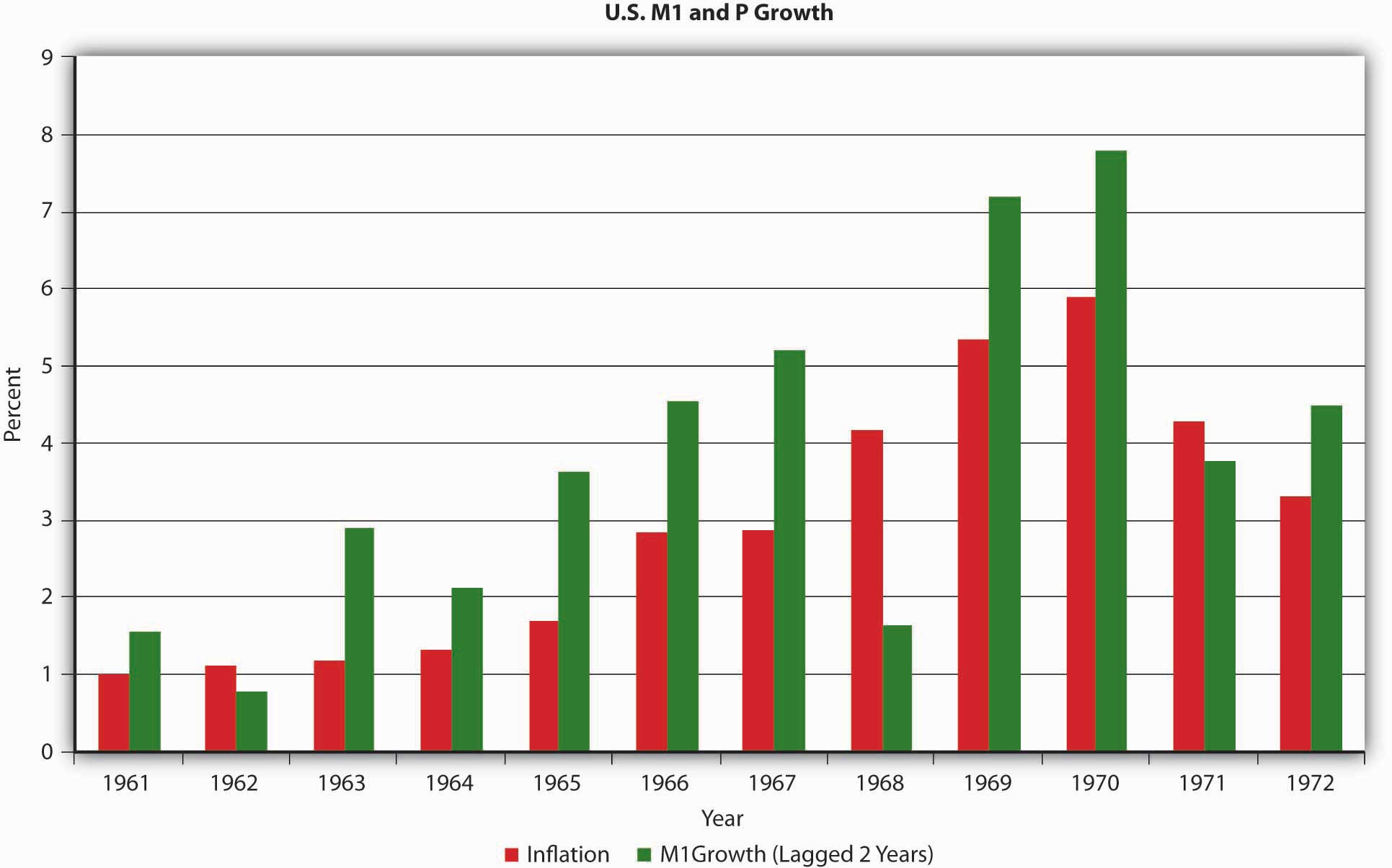
Figure 25.3 Government debt-to-GDP ratio
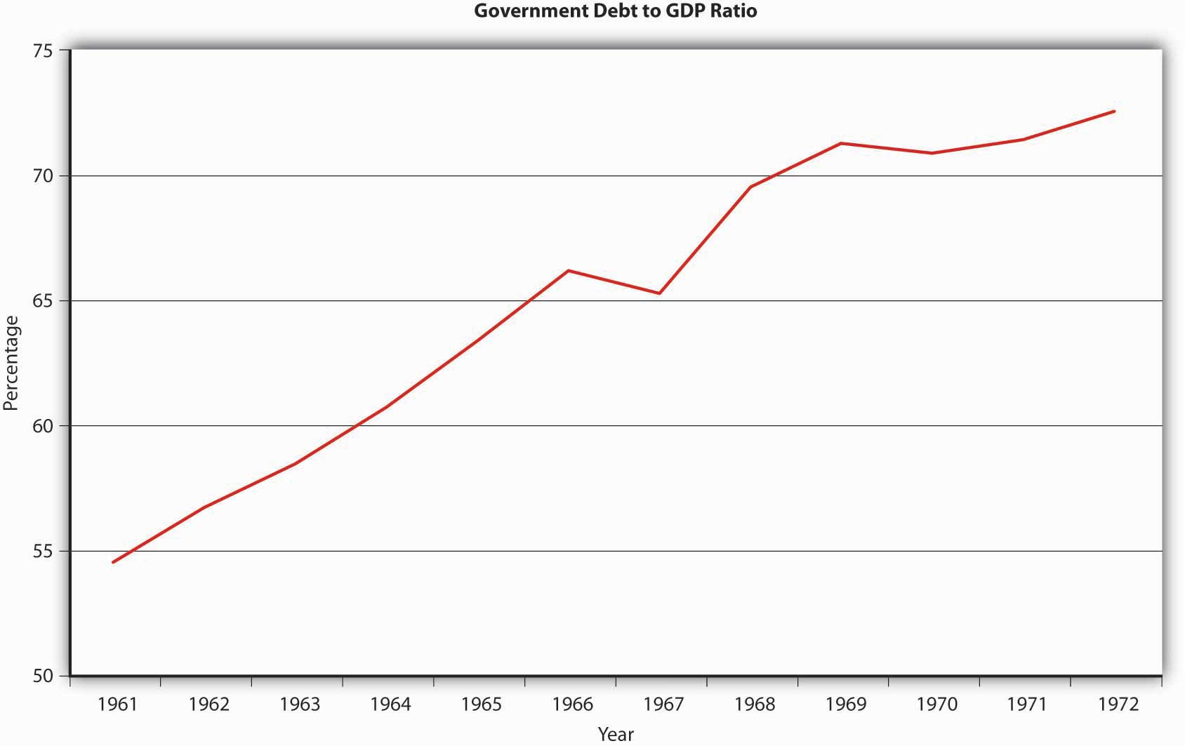
Figure 25.4 U.S. unemployment rates, 1961–1972
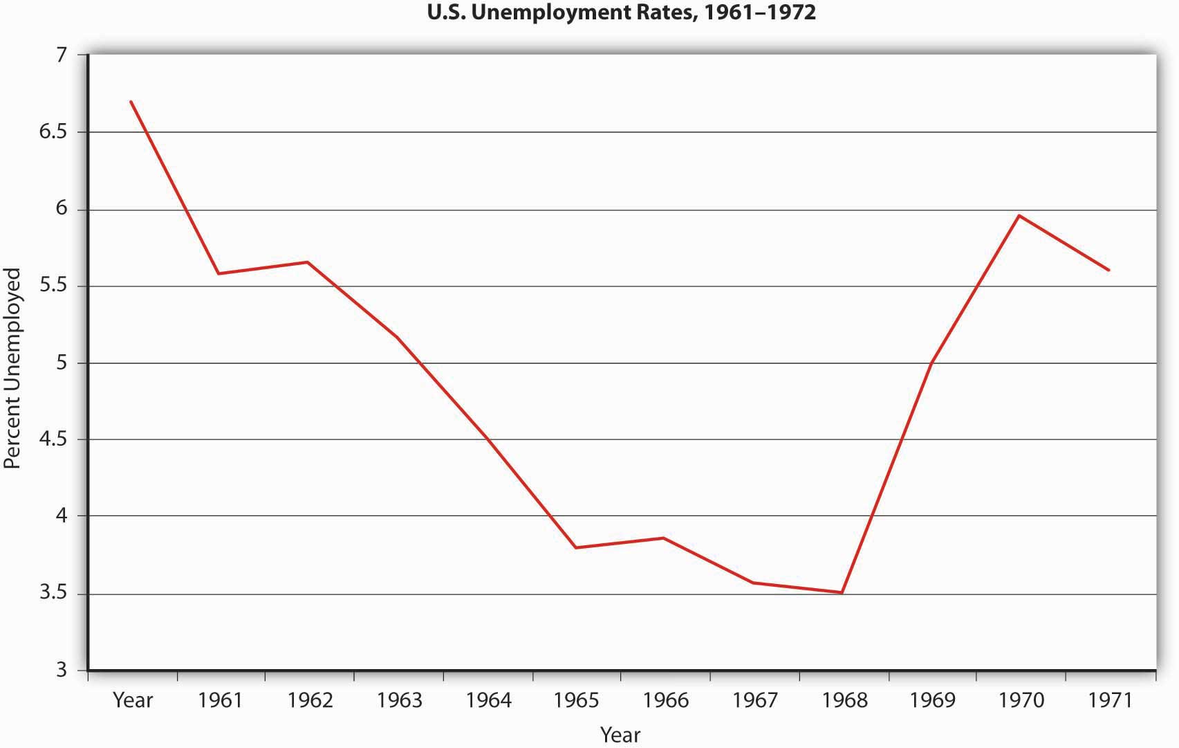
The data clearly show that M1 was growing over the period and likely causing inflation with a two-year lag. M1 grew partly because federal deficits increased faster than the economy, increasing the debt-to-GDP ratio, leading to debt monetization on the part of the Fed. Also, unemployment rates fell considerably below the natural rate of unemployment, suggesting that demand-pull inflation was taking place as well.
Key Takeaways
- Throughout history, exogenous increases in MS have led to increases in P*. Every hyperinflation has been preceded by rapid increases in money supply growth.
- The AS-AD model shows that money supply growth is the only thing that can lead to inflation, that is, sustained increases in the price level.
- This happens because monetary stimulus in the short term shifts the AD curve to the right, increasing prices but also rendering Y* > Ynrl.
- Unemployment drops, driving up wages, which shifts the AS curve to the left, Y* back to Ynrl, and P* yet higher.
- Unlike other variables, the MS can continue to grow, initiating round after round of this dynamic.
- Other variables are bounded and produce only one-off changes in P*.
- A negative supply shock or wage push, for instance, increases the price level once, but then price increases stop.
- Similarly, increases in government expenditures can cause P* to rise by shifting AD to the right, but unlike increases in the MS, government expenditures can increase only so far politically and practically (to 100 percent of GDP).
25.2 Why Have Central Bankers So Often Gotten It Wrong?
Learning Objectives
- Given the analysis in this chapter, why do central bankers sometimes allow inflation to occur year after year?
- What are lags and why are they important?
If the link between money supply growth and inflation is so clear, and if nobody (except perhaps inveterate debtors) has anything but contempt for inflation, why have central bankers allowed it to occur so frequently? Central bankers might be more privately interested than publicly interested and somehow benefit personally from inflation. (They might score points with politicians for stimulating the economy just before an election or they might take out big loans and repay them after the inflationary period in nearly worthless currency.) Assuming central bankers are publicly interested but far from prescient, what might cause them to err so often? In short, lags and high-employment policies.
A lag is an amount of time that passes between a cause and its eventual effect. Lags in monetary policy, Friedman showed, were “long and variable.” Data lag is the time it takes for policymakers to get important information, like GDP (Y) and unemployment. Recognition lag is the time it takes them to become convinced that the data is accurate and indicative of a trend and not just a random perturbation. Legislative lag is the time it takes legislators to react to economic changes. (This is short for monetary policy, but it can be a year or more for fiscal policy.) Implementation lag refers to the time between policy decision and implementation. (Again, for modern central banks using open market purchases (OMPs), this lag is minimal, but for changes in taxes, it can take a long time indeed.) The most important lag of all is the so-called effectiveness lag, the period between policy implementation and real-world results. All told, lags can add up to years and add considerable complexity to monetary policy analysis because they cloud cause-effect relationships. Lags also put policymakers perpetually behind the eight-ball, constantly playing catch-up. Lags force policymakers to forecast the future with accuracy, something (as we’ve seen) that is not easily done. As noted in earlier chapters, economists don’t even know when the short run becomes the long run!
Consider a case of so-called cost-push inflation brought about by a negative supply shock or wage push. That moves the AS curve to the left, reducing output and raising prices and, in all likelihood, causing unemployment and political angst. Policymakers unable to await the long term (the rightward shift in AS because Y* has fallen below Ynrl, causing unemployment and wages to decline) may well respond with what’s called accommodative monetary policy. In other words, they engage in expansionary monetary policies (EMPs), which shift the AD curve to the right, causing output to increase (with a lag) but prices to rise. Because prices are higher and they’ve been recently rewarded for their wage push with accommodative monetary policy, workers may well initiate another wage push, starting a vicious cycle of wage pushes followed by increases in P* and yet more wage pushes. Monetarists and other nonactivists shake their heads at this dynamic, arguing that if workers’ wage pushes were met by periods of higher unemployment, they would soon learn to stop. (After all, even 2-year-olds and rats eventually learn to stop pushing buttons if they are not rewarded for doing so. They learn even faster to stop pushing if they get a little shock.)
An episode of demand-pull inflation can also touch off accommodative monetary policy and a bout of inflation. If the government sets its full employment target too high, above the natural rate, it will always look like there is too much unemployment. That will eventually tempt policymakers into thinking that Y* is < Ynrl, inducing them to implement an EMP. Output will rise, temporarily, but so too will prices. Prices will go up again when the AS curve shifts left, back to Ynrl, as it will do in a hurry given the low level of unemployment. The shift, however, will again increase unemployment over the government’s unreasonably low target, inducing another round of EMP and price increases.
Another source of inflation is government budget deficits. To cover their expenditures, governments can tax, borrow at interest, or borrow for free by issuing money. (Which would you choose?) Taxation is politically costly. Borrowing at interest can be costly too, especially if the government is a default risk. Therefore, many governments pay their bills by printing money or by issuing bonds that their respective central banks then buy with money. Either way, the monetary base increases, leading to some multiple increases in the MS, which leads to inflation. Effectively a tax on money balances called a currency tax, inflation is easier to disguise and much easier to collect than other forms of taxes. Governments get as addicted to the currency tax as individuals get addicted to crack or meth. This is especially true in developing countries with weak (not independent) central banks.
Stop and Think Box
Why is central bank independence important in keeping inflation at bay?
Independent central banks are better able to withstand political pressures to monetize the debt, to follow accommodative policies, or to respond to (seemingly) “high” levels of unemployment with an EMP. They can also make a more believable or credible commitment to stop inflation, which (as we’ll see in Chapter 26 "Rational Expectations Redux: Monetary Policy Implications") is an important consideration as well.
Key Takeaways
- Private-interest scenarios aside, publicly interested central bankers might pursue high employment too vigorously, leading to inflation via cost-push and demand-pull mechanisms.
- If workers make a successful wage push, for example, the AS curve will shift left, increasing P*, decreasing Y*, and increasing unemployment.
- If policymakers are anxious to get out of recession, they might respond with an expansionary monetary policy (EMP).
- That will increase Y* but also P* yet again. Such an accommodative policy might induce workers to try another wage push. The price level is higher after all, and they were rewarded for their last wage push.
- The longer this dynamic occurs, the higher prices will go.
- Policymakers might fall into this trap themselves if they underestimate full employment at, say, 97 percent (3 percent unemployment) when in fact it is 95 percent (5 percent unemployment).
- Therefore, unemployment of 4 percent looks too high and output appears to be < Ynrl, suggesting that an EMP is in order.
- The rightward shift of the AD curve causes prices and output to rise, but the latter rises only temporarily as the already tight labor market gets tighter, leading to higher wages and a leftward shift of the AS curve, with its concomitant increase in P* and decrease in Y*.
- If policymakers’ original and flawed estimate of full employment is maintained, another round of AD is sure to come, as is higher prices.
- Budget deficits can also lead to sustained inflation if the government monetizes its debt directly by printing money (and deposits) or indirectly via central bank open market purchases (OMPs) of government bonds.
- Lags are the amount of time it takes between a change in the economy to take place and policymakers to effectively do something about it.
- That includes lags for gathering data, making sure the data show a trend and are not mere noise, making a legislative decision (if applicable), implementing policy (if applicable), and waiting for the policy to affect the economy.
- Lags are important because they are long and variable, thus complicating monetary policy by making central bankers play constant catch-up and also by clouding cause-effect relationships.
25.3 Suggested Reading
Ball, R. J. Inflation and the Theory of Money. Piscataway, NJ: Aldine Transaction, 2007.
Bresciani-Turroni, Costantino. Economics of Inflation. Auburn, AL: Ludwig von Mises Institute, 2007.
Samuelson, Robert. The Great Inflation and Its Aftermath: The Past and Future of American Affluence. New York: Random House, 2008.