This is “Risk Attitudes: Expected Utility Theory and Demand for Hedging”, chapter 3 from the book Enterprise and Individual Risk Management (v. 1.0). For details on it (including licensing), click here.
For more information on the source of this book, or why it is available for free, please see the project's home page. You can browse or download additional books there. To download a .zip file containing this book to use offline, simply click here.


Chapter 3 Risk Attitudes: Expected Utility Theory and Demand for Hedging
Authored by Puneet Prakash, Virginia Commonwealth University
Whenever we look into risks, risk measures, and risk management, we must always view these in a greater context. In this chapter, we focus on the risk within the “satisfaction” value maximization for individual and firms. The value here is measured economically. So, how do economists measure the value of satisfaction or happiness? Can we even measure satisfaction or happiness? Whatever the philosophical debate might be on the topic, economists have tried to measure the level of satisfaction.At one time, economists measured satisfaction in a unit called “utils” and discussed the highest number of utils as “bliss points”! What economists succeeded in doing is to compare levels of satisfaction an individual achieves when confronted with two or more choices. For example, we suppose that everyone likes to eat gourmet food at five-star hotels, drink French wine, vacation in exotic places, and drive luxury cars. For an economist, all these goods are assumed to provide satisfaction, some more than others. So while eating a meal at home gives us pleasure, eating exotic food at an upscale restaurant gives us an even higher level of satisfaction.
The problem with the quantity and quality of goods consumed is that we can find no common unit of measurement. That prevents economists from comparing levels of satisfaction from consumption of commodities that are different as apples are different from oranges. So does drinking tea give us the same type of satisfaction as eating cake? Or snorkeling as much as surfing?
To get around the problem of comparing values of satisfaction from noncomparable items, we express the value levels of satisfaction as a function of wealth. And indeed, we can understand intuitively that the level of wealth is linked directly to the quantity and quality of consumption a person can achieve. Notice the quality and level of consumption a person achieves is linked to the amount of wealth or to the individual’s budget. Economists consider that greater wealth can generate greater satisfaction. Therefore, a person with greater levels of wealth is deemed to be happier under the condition of everything else being equal between two individuals.Economists are fond of the phrase “ceteris paribus,” which means all else the same. We can only vary one component of human behavior at a time. We can link each person’s satisfaction level indirectly to that person’s wealth. The higher the person’s wealth, the greater his or her satisfaction level is likely to be.
Economists use the term “utils” to gauge a person’s satisfaction level. As a unit of measure, utils are similar to “ohms” as a measure of resistance in electrical engineering, except that utils cannot be measured with wires attached to a person’s head!
This notion that an individual derives satisfaction from wealth seems to work more often than not in economic situations. The economic theory that links the level of satisfaction to a person’s wealth level, and thus to consumption levels, is called utility theoryA theory postulated in economics to explain behavior of individuals based on the premise people can consistently rank order their choices depending upon their preferences.. Its basis revolves around individuals’ preferences, but we must use caution as we apply utility theory.The utility theory is utilized to compare two or more options. Thus, by its very nature, we refer to the utility theory as an “ordinal” theory, which rank orders choices, rather than “cardinal” utility, which has the ability to attach a number to even a single outcome where there are no choices involved.
In this chapter, we will study the utility theory. If utility theory is designed to measure satisfaction, and since every individual always tries to maximize satisfaction, it’s reasonable to expect (under utility theory) that each person tries to maximize his or her own utility.
Then we will extend utility to one of its logical extensions as applied to uncertain situations: expected utility (EU henceforth). So while utility theory deals with situations in which there is no uncertainty, the EU theory deals with choices individuals make when the outcomes they face are uncertain. As we shall see, if individuals maximize utility under certainty, they will also attempt to maximize EU under uncertainty.
However, individuals’ unabashed EU maximization is not always the case. Other models of human behavior describe behavior in which the observed choices of an individual vary with the decision rule to maximize EU. So why would a mother jump into a river to save her child, even if she does not know how to swim? Economists still confront these and other such questions. They have provided only limited answers to such questions thus far.
Hence, we will touch upon some uncertainty-laden situations wherein individuals’ observed behavior departs from the EU maximization principle. Systematic departures in behavior from the EU principle stem from “biases” that people exhibit, and we shall discuss some of these biases. Such rationales of observed behavior under uncertainty are termed “behavioral” explanations, rather than “rational” explanations—explanations that explore EU behavior of which economists are so fond.
In this chapter, we will apply the EU theory to individuals’ hedging decisions/purchase of insurance. Let’s start by asking, Why would anyone buy insurance? When most people face that question, they respond in one of three ways. One set says that insurance provides peace of mind (which we can equate to a level of satisfaction). Others respond more bluntly and argue that if it were not for regulation they’d never buy insurance. The second reply is one received mostly from younger adults. Still others posit that insurance is a “waste of money,” since they pay premiums up front and insurance never pays up in the absence of losses. To all those who argue based upon the third response, one might say, would they rather have a loss for the sake of recovering their premiums? We look to EU theory for some answers, and we will find that even if governments did not make purchase of insurance mandatory, the product would still have existed. Risk-averse individuals would always demand insurance for the peace of mind it confers.
Thus we will briefly touch upon the ways that insurance is useful, followed by a discussion of how some information problems affect the insurance industry more than any other industry. “Information asymmetry” problems arise, wherein one economic agent in a contract is better informed than the other party to the same contract. The study of information asymmetries has become a full-time occupation for some economics researchers. Notably, professors George A. Akerlof, A. Michael Spence, and Joseph E. Stiglitz were awarded the Nobel Prize in Economics in 2001 for their analyses of information asymmetry problems.
Links
Preferences are not absolute but rather they depend upon market conditions, cultures, peer groups, and surrounding events. Individuals’ preferences nestle within these parameters. Therefore, we can never talk in absolute terms when we talk about satisfaction and preferences. The 2008 crisis, which continued into 2009, provides a good example of how people’s preferences can change very quickly. When people sat around in celebration of 2009 New Year’s Eve, conversation centered on hopes for “making a living” and having some means for income. These same people talked about trips around the world at the end of 2007. Happiness and preferences are a dynamic topic depending upon individuals’ stage of life and economic states of the world. Under each new condition, new preferences arise that fall under the static utility theory discussed below. Economists have researched “happiness,” and continuing study is very important to economists.An academic example is the following study: Yew-Kwang Ng, “A Case for Happiness, Cardinalism, and Interpersonal Comparability,” Economic Journal 107 (1997): 1848–58. She contends that “modern economists are strongly biased in favour of preference (in contrast to happiness), ordinalism, and against interpersonal comparison. I wish to argue for the opposite.” A more popular research is at Forbes on happiness research.Forbes magazine published several short pieces on happiness research. Nothing especially rigorous, but a pleasant enough read: “Money Doesn’t Make People Happy,” by Tim Harford. But marriage, sex, socializing and even middle age do. http://www.forbes.com/2006/02/11/tim-harford-money_cz_th_money06_0214 harford.html “Shall I Compare Thee To A Summer’s Sausage?” by Daniel Gilbert. Money can’t make you happy, but making the right comparisons can. http://www.forbes.com/2006/02/11/daniel-gilbert-happiness_cx_dg_money06_0214 gilbert.html “Money, Happiness and the Pursuit of Both,” by Elizabeth MacDonald. When it comes [to] money and happiness, economists and psychologists have got it all wrong. http://www.forbes.com/2006/02/11/money-happiness-consumption_cz_em_money 06_0214pursuit.html “The Happiness Business,” by Paul Maidment. There is more academic research than you can shake a Havana cigar at saying there is no correlation between wealth and happiness. http://www.forbes.com/2006/02/11/happiness-economists-money_cx_pm_money 06_0214maidment.html
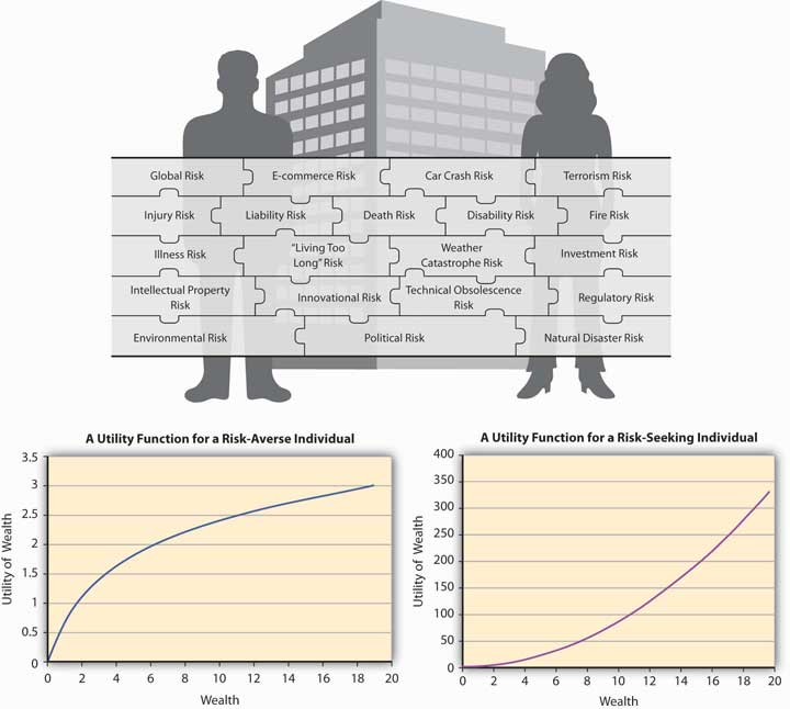
Figure 3.1 Links between the Holistic Risk Picture and Risk Attitudes
3.1 Utility Theory
Learning Objectives
- In this section we discuss economists’ utility theory.
- You will learn about assumptions that underlie individual preferences, which can then be mapped onto a utility “function,” reflecting the satisfaction level associated with individuals’ preferences.
- Further, we will explore how individuals maximize utility (or satisfaction).
Utility theoryA theory postulated in economics to explain behavior of individuals based on the premise people can consistently order rank their choices depending upon their preferences. bases its beliefs upon individuals’ preferences. It is a theory postulated in economics to explain behavior of individuals based on the premise people can consistently rank order their choices depending upon their preferences. Each individual will show different preferences, which appear to be hard-wired within each individual. We can thus state that individuals’ preferences are intrinsic. Any theory, which proposes to capture preferences, is, by necessity, abstraction based on certain assumptions. Utility theory is a positive theoryTheory that seeks to explain an individual’s observed behavior and choices. that seeks to explain the individuals’ observed behavior and choices.The distinction between normative and positive aspects of a theory is very important in the discipline of economics. Some people argue that economic theories should be normative, which means they should be prescriptive and tell people what to do. Others argue, often successfully, that economic theories are designed to be explanations of observed behavior of agents in the market, hence positive in that sense. This contrasts with a normative theoryTheory that dictates that people should behave in the manner prescribed by it., one that dictates that people should behave in the manner prescribed by it. Instead, it is only since the theory itself is positive, after observing the choices that individuals make, we can draw inferences about their preferences. When we place certain restrictions on those preferences, we can represent them analytically using a utility functionA mathematical formulation that ranks the preferences of the individual in terms of satisfaction different consumption bundles provide.—a mathematical formulation that ranks the preferences of the individual in terms of satisfaction different consumption bundles provide. Thus, under the assumptions of utility theory, we can assume that people behaved as if they had a utility function and acted according to it. Therefore, the fact that a person does not know his/her utility function, or even denies its existence, does not contradict the theory. Economists have used experiments to decipher individuals’ utility functions and the behavior that underlies individuals’ utility.
To begin, assume that an individual faces a set of consumption “bundles.” We assume that individuals have clear preferences that enable them to “rank order” all bundles based on desirability, that is, the level of satisfaction each bundle shall provide to each individual. This rank ordering based on preferences tells us the theory itself has ordinal utilityUtility that can only represent relative levels of satisfaction between two or more alternatives, that is, rank orders them.—it is designed to study relative satisfaction levels. As we noted earlier, absolute satisfaction depends upon conditions; thus, the theory by default cannot have cardinal utilityUtility that can represent the absolute level of satisfaction., or utility that can represent the absolute level of satisfaction. To make this theory concrete, imagine that consumption bundles comprise food and clothing for a week in all different combinations, that is, food for half a week, clothing for half a week, and all other possible combinations.
The utility theory then makes the following assumptions:
- Completeness: Individuals can rank order all possible bundles. Rank ordering implies that the theory assumes that, no matter how many combinations of consumption bundles are placed in front of the individual, each individual can always rank them in some order based on preferences. This, in turn, means that individuals can somehow compare any bundle with any other bundle and rank them in order of the satisfaction each bundle provides. So in our example, half a week of food and clothing can be compared to one week of food alone, one week of clothing alone, or any such combination. Mathematically, this property wherein an individual’s preferences enable him or her to compare any given bundle with any other bundle is called the completenessProperty in which an individual’s preferences enable him/her to compare any given consumption bundle with any other bundle. property of preferences.
- More-is-better: Assume an individual prefers consumption of bundle A of goods to bundle B. Then he is offered another bundle, which contains more of everything in bundle A, that is, the new bundle is represented by αA where α = 1. The more-is-better assumption says that individuals prefer αA to A, which in turn is preferred to B, but also A itself. For our example, if one week of food is preferred to one week of clothing, then two weeks of food is a preferred package to one week of food. Mathematically, the more-is-better assumption is called the monotonicity assumptionThe assumption that more consumption is always better. on preferences. One can always argue that this assumption breaks down frequently. It is not difficult to imagine that a person whose stomach is full would turn down additional food. However, this situation is easily resolved. Suppose the individual is given the option of disposing of the additional food to another person or charity of his or her choice. In this case, the person will still prefer more food even if he or she has eaten enough. Thus under the monotonicity assumption, a hidden property allows costless disposal of excess quantities of any bundle.
- Mix-is-better: Suppose an individual is indifferent to the choice between one week of clothing alone and one week of food. Thus, either choice by itself is not preferred over the other. The “mix-is-better” assumptionThe assumption that a mix of consumption bundles is always better than stand-alone choices. about preferences says that a mix of the two, say half-week of food mixed with half-week of clothing, will be preferred to both stand-alone choices. Thus, a glass of milk mixed with Milo (Nestlè’s drink mix), will be preferred to milk or Milo alone. The mix-is-better assumption is called the “convexity” assumption on preferences, that is, preferences are convex.
- Rationality: This is the most important and controversial assumption that underlies all of utility theory. Under the assumption of rationalityThe assumption that individuals’ preferences avoid any kind of circularity., individuals’ preferences avoid any kind of circularity; that is, if bundle A is preferred to B, and bundle B is preferred to C, then A is also preferred to C. Under no circumstances will the individual prefer C to A. You can likely see why this assumption is controversial. It assumes that the innate preferences (rank orderings of bundles of goods) are fixed, regardless of the context and time.
If one thinks of preference orderings as comparative relationships, then it becomes simpler to construct examples where this assumption is violated. So, in “beats”—as in A beat B in college football. These are relationships that are easy to see. For example, if University of Florida beats Ohio State, and Ohio State beats Georgia Tech, it does not mean that Florida beats Georgia Tech. Despite the restrictive nature of the assumption, it is a critical one. In mathematics, it is called the assumption of transitivity of preferences.
Whenever these four assumptions are satisfied, then the preferences of the individual can be represented by a well-behaved utility functionA representation of the preferences of the individual that satisfies the assumptions of completeness, monotonicity, mix-is-better, and rationality..The assumption of convexity of preferences is not required for a utility function representation of an individual’s preferences to exist. But it is necessary if we want that function to be well behaved. Note that the assumptions lead to “a” function, not “the” function. Therefore, the way that individuals represent preferences under a particular utility function may not be unique. Well-behaved utility functions explain why any comparison of individual people’s utility functions may be a futile exercise (and the notion of cardinal utility misleading). Nonetheless, utility functions are valuable tools for representing the preferences of an individual, provided the four assumptions stated above are satisfied. For the remainder of the chapter we will assume that preferences of any individual can always be represented by a well-behaved utility function. As we mentioned earlier, well-behaved utility depends upon the amount of wealth the person owns.
Utility theory rests upon the idea that people behave as if they make decisions by assigning imaginary utility values to the original monetary values. The decision maker sees different levels of monetary values, translates these values into different, hypothetical terms (“utils”), processes the decision in utility terms (not in wealth terms), and translates the result back to monetary terms. So while we observe inputs to and results of the decision in monetary terms, the decision itself is made in utility terms. And given that utility denotes levels of satisfaction, individuals behave as if they maximize the utility, not the level of observed dollar amounts.
While this may seem counterintuitive, let’s look at an example that will enable us to appreciate this distinction better. More importantly, it demonstrates why utility maximization, rather than wealth maximization, is a viable objective. The example is called the “St. Petersburg paradox.” But before we turn to that example, we need to review some preliminaries of uncertainty: probability and statistics.
Key Takeaways
- In economics, utility theory governs individual decision making. The student must understand an intuitive explanation for the assumptions: completeness, monotonicity, mix-is-better, and rationality (also called transitivity).
- Finally, students should be able to discuss and distinguish between the various assumptions underlying the utility function.
Discussion Questions
- Utility theory is a preference-based approach that provides a rank ordering of choices. Explain this statement.
- List and describe in your own words the four axioms/assumptions that lead to the existence of a utility function.
- What is a “util” and what does it measure?
3.2 Uncertainty, Expected Value, and Fair Games
Learning Objectives
- In this section we discuss the notion of uncertainty. Mathematical preliminaries discussed in this section form the basis for analysis of individual decision making in uncertain situations.
- The student should pick up the tools of this section, as we will apply them later.
As we learned in the chapters Chapter 1 "The Nature of Risk: Losses and Opportunities" and Chapter 2 "Risk Measurement and Metrics", risk and uncertainty depend upon one another. The origins of the distinction go back to the Mr. Knight,See Jochen Runde, “Clarifying Frank Knight’s Discussion of the Meaning of Risk and Uncertainty,” Cambridge Journal of Economics 22, no. 5 (1998): 539–46. who distinguished between risk and uncertainty, arguing that measurable uncertainty is risk. In this section, since we focus only on measurable uncertainty, we will not distinguish between risk and uncertainty and use the two terms interchangeably.
As we described in Chapter 2 "Risk Measurement and Metrics", the study of uncertainty originated in games of chance. So when we play games of dice, we are dealing with outcomes that are inherently uncertain. The branch of science of uncertain outcomes is probability and statistics. Notice that the analysis of probability and statistics applies only if outcomes are uncertain. When a student registers for a class but does not attend any lectures nor does any assigned work or test, only one outcome is possible: a failing grade. On the other hand, if the student attends all classes and scores 100 percent on all tests and assignments, then too only one outcome is possible, an “A” grade. In these extreme situations, no uncertainty arises with the outcomes. But between these two extremes lies the world of uncertainty. Students often do research on the instructor and try to get a “feel” for the chance that they will make a particular grade if they register for an instructor’s course.
Even though we covered some of this discussion of probability and uncertainty in Chapter 2 "Risk Measurement and Metrics", we repeat it here for reinforcement. Figuring out the chance, in mathematical terms, is the same as calculating the probability of an event. To compute a probability empirically, we repeat an experiment with uncertain outcomes (called a random experiment) and count the number of times the event of interest happens, say n, in the N trials of the experiment. The empirical probability of the event then equals n/N. So, if one keeps a log of the number of times a computer crashes in a day and records it for 365 days, the probability of the computer crashing on a day will be the sum of all of computer crashes on a daily basis (including zeroes for days it does not crash at all) divided by 365.
For some problems, the probability can be calculated using mathematical deduction. In these cases, we can figure out the probability of getting a head on a coin toss, two aces when two cards are randomly chosen from a deck of 52 cards, and so on (see the example of the dice in Chapter 2 "Risk Measurement and Metrics"). We don’t have to conduct a random experiment to actually compute the mathematical probability, as is the case with empirical probability.
Finally, as strongly suggested before, subjective probability is based on a person’s beliefs and experiences, as opposed to empirical or mathematical probability. It may also depend upon a person’s state of mind. Since beliefs may not always be rational, studying behavior using subjective probabilities belongs to the realm of behavioral economics rather than traditional rationality-based economics.
So consider a lottery (a game of chance) wherein several outcomes are possible with defined probabilities. Typically, outcomes in a lottery consist of monetary prizes. Returning to our dice example of Chapter 2 "Risk Measurement and Metrics", let’s say that when a six-faced die is rolled, the payoffs associated with the outcomes are $1 if a 1 turns up, $2 for a 2, …, and $6 for a 6. Now if this game is played once, one and only one amount can be won—$1, $2, and so on. However, if the same game is played many times, what is the amount that one can expect to win?
Mathematically, the answer to any such question is very straightforward and is given by the expected value of the game.
In a game of chance, if are the N outcomes possible with probabilities , then the expected value of the game (G) is
The computation can be extended to expected values of any uncertain situation, say losses, provided we know the outcome numbers and their associated probabilities. The probabilities sum to 1, that is,
While the computation of expected value is important, equally important is notion behind expected values. Note that we said that when it comes to the outcome of a single game, only one amount can be won, either $1, $2, …, $6. But if the game is played over and over again, then one can expect to win per game. Often—like in this case—the expected value is not one of the possible outcomes of the distribution. In other words, the probability of getting $3.50 in the above lottery is zero. Therefore, the concept of expected value is a long-run concept, and the hidden assumption is that the lottery is played many times. Secondly, the expected valueThe sum of the products of two numbers, the outcomes and their associated probabilities. is a sum of the products of two numbers, the outcomes and their associated probabilities. If the probability of a large outcome is very high then the expected value will also be high, and vice versa.
Expected value of the game is employed when one designs a fair gameGame in which the cost of playing equals the expected winnings of the game, so that net value of the game equals zero.. A fair game, actuarially speaking, is one in which the cost of playing the game equals the expected winnings of the game, so that net value of the game equals zero. We would expect that people are willing to play all fair value games. But in practice, this is not the case. I will not pay $500 for a lucky outcome based on a coin toss, even if the expected gains equal $500. No game illustrates this point better than the St. Petersburg paradox.
The paradox lies in a proposed game wherein a coin is tossed until “head” comes up. That is when the game ends. The payoff from the game is the following: if head appears on the first toss, then $2 is paid to the player, if it appears on the second toss then $4 is paid, if it appears on the third toss, then $8, and so on, so that if head appears on the nth toss then the payout is $2n. The question is how much would an individual pay to play this game?
Let us try and apply the fair value principle to this game, so that the cost an individual is willing to bear should equal the fair value of the game. The expected value of the game E(G) is calculated below.
The game can go on indefinitely, since the head may never come up in the first million or billion trials. However, let us look at the expected payoff from the game. If head appears on the first try, the probability of that happening is and the payout is $2. If it happens on the second try, it means the first toss yielded a tail (T) and the second a head (H). The probability of TH combination and the payoff is $4. Then if H turns up on the third attempt, it implies the sequence of outcomes is TTH, and the probability of that occurring is with a payoff of $8. We can continue with this inductive analysis ad infinitum. Since expected is the sum of all products of outcomes and their corresponding probabilities,
It is evident that while the expected value of the game is infinite, not even the Bill Gateses and Warren Buffets of the world will give even a thousand dollars to play this game, let alone billions.
Daniel Bernoulli was the first one to provide a solution to this paradox in the eighteenth century. His solution was that individuals do not look at the expected wealth when they bid a lottery price, but the expected utility of the lottery is the key. Thus, while the expected wealth from the lottery may be infinite, the expected utility it provides may be finite. Bernoulli termed this as the “moral value” of the game. Mathematically, Bernoulli’s idea can be expressed with a utility function, which provides a representation of the satisfaction level the lottery provides.
Bernoulli used to represent the utility that this lottery provides to an individual where W is the payoff associated with each event H, TH, TTH, and so on, then the expected utility from the game is given by
which can be shown to equal 1.39 after some algebraic manipulation. Since the expected utility that this lottery provides is finite (even if the expected wealth is infinite), individuals will be willing to pay only a finite cost for playing this lottery.
The next logical question to ask is, What if the utility was not given as natural log of wealth by Bernoulli but something else? What is that about the natural log function that leads to a finite expected utility? This brings us to the issue of expected utility and its central place in decision making under uncertainty in economics.
Key Takeaways
- Students should be able to explain probability as a measure of uncertainty in their own words.
- Moreover, the student should also be able to explain that any expected value is the sum of product of probabilities and outcomes and be able to compute expected values.
Discussion Questions
- Define probability. In how many ways can one come up with a probability estimate of an event? Describe.
- Explain the need for utility functions using St. Petersburg paradox as an example.
- Suppose a six-faced fair die with numbers 1–6 is rolled. What is the number you expect to obtain?
- What is an actuarially fair game?
3.3 Choice under Uncertainty: Expected Utility Theory
Learning Objectives
- In this section the student learns that an individual’s objective is to maximize expected utility when making decisions under uncertainty.
- We also learn that people are risk averse, risk neutral, or risk seeking (loving).
We saw earlier that in a certain world, people like to maximize utility. In a world of uncertainty, it seems intuitive that individuals would maximize expected utilityA construct to explain the level of satisfaction a person gets when faced with uncertain choices.. This refers to a construct used to explain the level of satisfaction a person gets when faced with uncertain choices. The intuition is straightforward, proving it axiomatically was a very challenging task. John von Neumann and Oskar Morgenstern (1944) advocated an approach that leads us to a formal mathematical representation of maximization of expected utility.
We have also seen that a utility function representation exists if the four assumptions discussed above hold. Messrs. von Neumann and Morgenstern added two more assumptions and came up with an expected utility function that exists if these axioms hold. While the discussions about these assumptionsThese are called the continuity and independence assumptions. is beyond the scope of the text, it suffices to say that the expected utility function has the form
where u is a function that attaches numbers measuring the level of satisfaction ui associated with each outcome i. u is called the Bernoulli function while E(U) is the von Neumann-Morgenstern expected utility function.
Again, note that expected utility function is not unique, but several functions can model the preferences of the same individual over a given set of uncertain choices or games. What matters is that such a function (which reflects an individual’s preferences over uncertain games) exists. The expected utility theory then says if the axioms provided by von Neumann-Morgenstern are satisfied, then the individuals behave as if they were trying to maximize the expected utility.
The most important insight of the theory is that the expected value of the dollar outcomes may provide a ranking of choices different from those given by expected utility. The expected utility theoryTheory that says persons will choose an option that maximizes their expected utility rather than their expected wealth. then says persons shall choose an option (a game of chance or lottery) that maximizes their expected utility rather than the expected wealth. That expected utility ranking differs from expected wealth ranking is best explained using the example below.
Let us think about an individual whose utility function is given by and has an initial endowment of $10. This person faces the following three lotteries, based on a coin toss:
Table 3.1 Utility Function with Initial Endowment of $10
| Outcome (Probability) | Payoff Lottery 1 | Payoff Lottery 2 | Payoff Lottery 3 |
|---|---|---|---|
| H (0.5) | 10 | 20 | 30 |
| T (0.5) | −2 | −5 | −10 |
| E(G) | 4 | 7.5 | 10 |
We can calculate the expected payoff of each lottery by taking the product of probability and the payoff associated with each outcome and summing this product over all outcomes. The ranking of the lotteries based on expected dollar winnings is lottery 3, 2, and 1—in that order. But let us consider the ranking of the same lotteries by this person who ranks them in order based on expected utility.
We compute expected utility by taking the product of probability and the associated utility corresponding to each outcome for all lotteries. When the payoff is $10, the final wealth equals initial endowment ($10) plus winnings = ($20). The utility of this final wealth is given by The completed utility table is shown below.
Table 3.2 Lottery Rankings by Expected Utility
| Outcome (Probability) | Utility Lottery 1 | Utility Lottery 2 | Utility Lottery 3 |
|---|---|---|---|
| H (0.5) | 4.472 | 5.477 | 6.324 |
| T (0.5) | 2.828 | 2.236 | 0 |
| E(U) = | 3.650 | 3.856 | 3.162 |
The expected utility ranks the lotteries in the order 2–1–3. So the expected utility maximization principle leads to choices that differ from the expected wealth choices.
The example shows that the ranking of games of chance differs when one utilizes the expected utility (E[U]) theory than when the expected gain E(G) principle applies This leads us to the insight that if two lotteries provide the same E(G), the expected gain principle will rank both lotteries equally, while the E(U) theory may lead to unique rankings of the two lotteries. What happens when the E(U) theory leads to a same ranking? The theory says the person is indifferent between the two lotteries.
Risk Types and Their Utility Function Representations
What characteristic of the games of chance can lead to same E(G) but different E(U)? The characteristic is the “risk” associated with each game.At this juncture, we only care about that notion of risk, which captures the inherent variability in the outcomes (uncertainty) associated with each lottery. Then the E(U) theory predicts that the individuals’ risk “attitude” for each lottery may lead to different rankings between lotteries. Moreover, the theory is “robust” in the sense that it also allows for attitudes toward risk to vary from one individual to the next. As we shall now see, the E(U) theory does enable us to capture different risk attitudes of individuals. Technically, the difference in risk attitudes across individuals is called “heterogeneity of risk preferences” among economic agents.
From the E(U) theory perspective, we can categorize all economic agents into one of the three categories as noted in Chapter 1 "The Nature of Risk: Losses and Opportunities":
- Risk averse
- Risk neutral
- Risk seeking (or loving)
We will explore how E(U) captures these attitudes and the meaning of each risk attitude next.
Consider the E(U) function given by Let the preferences be such that the addition to utility one gets out of an additional dollar at lower levels of wealth is always greater than the additional utility of an extra dollar at higher levels of wealth. So, let us say that when a person has zero wealth (no money), then the person has zero utility. Now if the person receives a dollar, his utility jumps to 1 util. If this person is now given an additional dollar, then as per the monotonicity (more-is-better) assumption, his utility will go up. Let us say that it goes up to 1.414 utils so that the increase in utility is only 0.414 utils, while earlier it was a whole unit (1 util). At 2 dollars of wealth, if the individual receives another dollar, then again his families’ utility rises to a new level, but only to 1.732 utils, an increase of 0.318 units (1.732 − 1.414). This is increasing utility at a decreasing rate for each additional unit of wealth. Figure 3.2 "A Utility Function for a Risk-Averse Individual" shows a graph of the utility.
Figure 3.2 A Utility Function for a Risk-Averse Individual
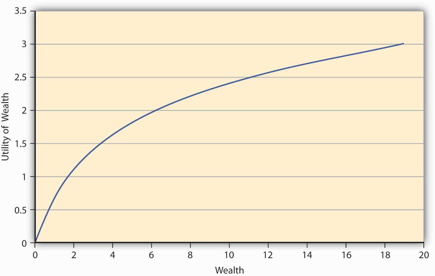
The first thing we notice from Figure 3.2 "A Utility Function for a Risk-Averse Individual" is its concavityProperty of a curve in which a chord connecting any two points on the curve will lie strictly below the curve., which means if one draws a chord connecting any two points on the curve, the chord will lie strictly below the curve. Moreover, the utility is always increasing although at a decreasing rate. This feature of this particular utility function is called diminishing marginal utilityFeature of a utility function in which utility is always increasing although at a decreasing rate.. Marginal utility at any given wealth level is nothing but the slope of the utility function at that wealth level.Mathematically, the property that the utility is increasing at a decreasing rate can be written as a combination of restrictions on the first and second derivatives (rate of change of slope) of the utility function, Some functions that satisfy this property are The functional form depicted in Figure 3.2 "A Utility Function for a Risk-Averse Individual" is LN(W).
The question we ask ourselves now is whether such an individual, whose utility function has the shape in Figure 3.2 "A Utility Function for a Risk-Averse Individual", will be willing to pay the actuarially fair price (AFP)The expected loss in wealth to the individual., which equals expected winnings, to play a game of chance? Let the game that offers him payoffs be offered to him. In Game 1, tables have playoff games by Game 1 in Table 3.1 "Utility Function with Initial Endowment of $10" based on the toss of a coin. The AFP for the game is $4. Suppose that a person named Terry bears this cost upfront and wins; then his final wealth is $10 − $4 + $10 = $16 (original wealth minus the cost of the game, plus the winning of $10), or else it equals $10 − $4 − $2 = $4 (original wealth minus the cost of the game, minus the loss of $2) in case he loses. Let the utility function of this individual be given by Then expected utility when the game costs AFP equals utils. On the other hand, suppose Terry doesn’t play the game; his utility remains at Since the utility is higher when Terry doesn’t play the game, we conclude that any individual whose preferences are depicted by Figure 3.2 "A Utility Function for a Risk-Averse Individual" will forgo a game of chance if its cost equals AFP. This is an important result for a concave utility function as shown in Figure 3.2 "A Utility Function for a Risk-Averse Individual".
Such a person will need incentives to be willing to play the game. It could come as a price reduction for playing the lottery, or as a premium that compensates the individual for risk. If Terry already faces a risk, he will pay an amount greater than the actuarially fair value to reduce or eliminate the risk. Thus, it works both ways—consumers demand a premium above AFP to take on risk. Just so, insurance companies charge individuals premiums for risk transfer via insurances.
An individual—let’s name him Johann—has preferences that are characterized by those shown in Figure 3.2 "A Utility Function for a Risk-Averse Individual" (i.e., by a concave or diminishing marginal utility function). Johann is a risk-averse person. We have seen that a risk-averse person refuses to play an actuarially fair game. Such risk aversions also provide a natural incentive for Johann to demand (or, equivalently, pay) a risk premium above AFP to take on (or, equivalently, get rid of) risk. Perhaps you will recall from Chapter 1 "The Nature of Risk: Losses and Opportunities" that introduced a more mathematical measure to the description of risk aversion. In an experimental study, Holt and Laury (2002) find that a majority of their subjects under study made “safe choices,” that is, displayed risk aversion. Since real-life situations can be riskier than laboratory settings, we can safely assume that a majority of people are risk averse most of the time. What about the remainder of the population?
We know that most of us do not behave as risk-averse people all the time. In the later 1990s, the stock market was considered to be a “bubble,” and many people invested in the stock market despite the preferences they exhibited before this time. At the time, Federal Reserve Board Chairman Alan Greenspan introduced the term “irrational exuberance” in a speech given at the American Enterprise Institute. The phrase has become a regular way to describe people’s deviations from normal preferences. Such behavior was also repeated in the early to mid-2000s with a real estate bubble. People without the rational means to buy homes bought them and took “nonconventional risks,” which led to the 2008–2009 financial and credit crisis and major recessions (perhaps even depression) as President Obama took office in January 2009. We can regard external market conditions and the “herd mentality” to be significant contributors to changing rational risk aversion traits.
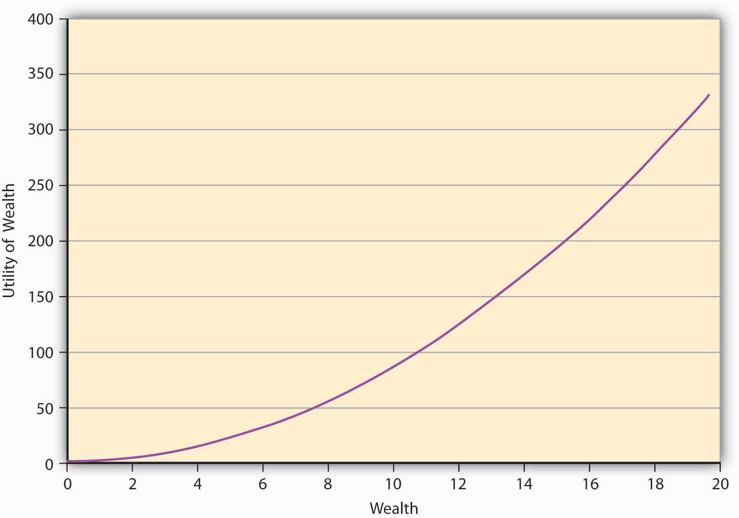
An individual may go skydiving, hang gliding, and participate in high-risk-taking behavior. Our question is, can the expected utility theory capture that behavior as well? Indeed it can, and that brings us to risk-seeking behavior and its characterization in E(U) theory. Since risk-seeking behavior exhibits preferences that seem to be the opposite of risk aversion, the mathematical functional representation may likewise show opposite behavior. For a risk-loving person, the utility function will show the shape given in Figure 3.3 "A Utility Function for a Risk-Seeking Individual". It shows that the greater the level of wealth of the individual, the higher is the increase in utility when an additional dollar is given to the person. We call this feature of the function, in which utility is always increasing at an increasing rate, increasing marginal utilityFeature of a utility function in which utility is always increasing at an increasing rate.. It turns out that all convex utility functionsUtility function in which the curve lies strictly below the chord joining any two points on the curve. look like Figure 3.3 "A Utility Function for a Risk-Seeking Individual". The curve lies strictly below the chord joining any two points on the curve.The convex curve in Figure 3.2 "A Utility Function for a Risk-Averse Individual" has some examples that include the mathematical function .
Figure 3.3 A Utility Function for a Risk-Seeking Individual
A risk-seeking individual will always choose to play a gamble at its AFP. For example, let us assume that the individual’s preferences are given by As before, the individual owns $10, and has to decide whether or not to play a lottery based on a coin toss. The payoff if a head turns up is $10 and −$2 if it’s a tail. We have seen earlier (in Table 3.1 "Utility Function with Initial Endowment of $10") that the AFP for playing this lottery is $4.
The expected utility calculation is as follows. After bearing the cost of the lottery upfront, the wealth is $6. If heads turns up, the final wealth becomes $16 ($6 + $10). In case tails turns face-up, then the final wealth equals $4 ($6 − $2). People’s expected utility if they play the lottery is utils.
On the other hand, if an individual named Ray decides not to play the lottery, then the Since the E(U) is higher if Ray plays the lottery at its AFP, he will play the lottery. As a matter of fact, this is the mind-set of gamblers. This is why we see so many people at the slot machines in gambling houses.
The contrast between the choices made by risk-averse individuals and risk-seeking individuals is starkly clear in the above example.Mathematically speaking, for a risk-averse person, we have Similarly, for a risk-seeking person we have This result is called Jensen’s inequality. To summarize, a risk-seeking individual always plays the lottery at its AFP, while a risk-averse person always forgoes it. Their concave (Figure 3.1 "Links between the Holistic Risk Picture and Risk Attitudes") versus convex (Figure 3.2 "A Utility Function for a Risk-Averse Individual") utility functions and their implications lie at the heart of their decision making.
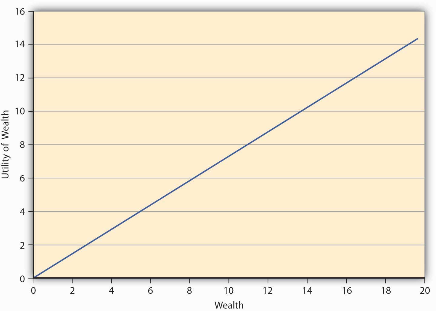
Finally, we come to the third risk attitude type wherein an individual is indifferent between playing a lottery and not playing it. Such an individual is called risk neutral. The preferences of such an individual can be captured in E(U) theory by a linear utility function of the form where a is a real number > 0. Such an individual gains a constant marginal utility of wealth, that is, each additional dollar adds the same utility to the person regardless of whether the individual is endowed with $10 or $10,000. The utility function of such an individual is depicted in Figure 3.4 "A Utility Function for a Risk-Neutral Individual".
Figure 3.4 A Utility Function for a Risk-Neutral Individual
Key Takeaways
- This section lays the foundation for analysis of individuals’ behavior under uncertainty. Student should be able to describe it as such.
- The student should be able to compute expected gains and expected utilities.
- Finally, and most importantly, the concavity and convexity of the utility function is key to distinguishing between risk-averse and risk-seeking individuals.
Discussion Questions
- Discuss the von Neumann-Morgenstern expected utility function and discuss how it differs from expected gains.
- You are told that is a utility function with diminishing marginal utility. Is it correct? Discuss, using definition of diminishing marginal utility.
- An individual has a utility function given by and initial wealth of $100. If he plays a costless lottery in which he can win or lose $10 at the flip of a coin, compute his expected utility. What is the expected gain? Will such a person be categorized as risk neutral?
- Discuss the three risk types with respect to their shapes, technical/mathematical formulation, and the economic interpretation.
3.4 Biases Affecting Choice under Uncertainty
Learning Objective
- In this section the student learns that an individual’s behavior cannot always be characterized within an expected utility framework. Biases and other behavioral aspects make individuals deviate from the behavior predicted by the E(U) theory.
Why do some people jump into the river to save their loved ones, even if they cannot swim? Why would mothers give away all their food to their children? Why do we have herd mentality where many individuals invest in the stock market at times of bubbles like at the latter part of the 1990s? These are examples of aspects of human behavior that E(U) theory fails to capture. Undoubtedly, an emotional component arises to explain the few examples given above. Of course, students can provide many more examples. The realm of academic study that deals with departures from E(U) maximization behavior is called behavioral economicsRealm of academic study that deals with departures from E(U) maximization behavior..
While expected utility theory provides a valuable tool for analyzing how rational people should make decisions under uncertainty, the observed behavior may not always bear it out. Daniel Kahneman and Amos Tversky (1974) were the first to provide evidence that E(U) theory doesn’t provide a complete description of how people actually decide under uncertain conditions. The authors conducted experiments that demonstrate this variance from the E(U) theory, and these experiments have withstood the test of time. It turns out that individual behavior under some circumstances violates the axioms of rational choice of E(U) theory.
Kahneman and Tversky (1981) provide the following example: Suppose the country is going to be struck by the avian influenza (bird flu) pandemic. Two programs are available to tackle the pandemic, A and B. Two sets of physicians, X and Y, are set with the task of containing the disease. Each group has the outcomes that the two programs will generate. However, the outcomes have different phrasing for each group. Group X is told about the efficacy of the programs in the following words:
- Program A: If adopted, it will save exactly 200 out of 600 patients.
- Program B: If adopted, the probability that 600 people will be saved is 1/3, while the probability that no one will be saved is 2/3.
Seventy-six percent of the doctors in group X chose to administer program A.
Group Y, on the other hand, is told about the efficacy of the programs in these words:
- Program A: If adopted, exactly 400 out of 600 patients will die.
- Program B: If adopted, the probability that nobody will die is 1/3, while the probability that all 600 will die is 2/3.
Only 13 percent of the doctors in this group chose to administer program A.
The only difference between the two sets presented to groups X and Y is the description of the outcomes. Every outcome to group X is defined in terms of “saving lives,” while for group Y it is in terms of how many will “die.” Doctors, being who they are, have a bias toward “saving” lives, naturally.
This experiment has been repeated several times with different subjects and the outcome has always been the same, even if the numbers differ. Other experiments with different groups of people also showed that the way alternatives are worded result in different choices among groups. The coding of alternatives that makes individuals vary from E(U) maximizing behavior is called the framing effectThe coding of alternatives, which makes individuals vary from E(U) maximizing behavior..
In order to explain these deviations from E(U), Kahneman and Tversky suggest that individuals use a value functionA mathematical formulation that seeks to explain observed behavior without making any assumption about preferences. to assess alternatives. This is a mathematical formulation that seeks to explain observed behavior without making any assumption about preferences. The nature of the value function is such that it is much steeper in losses than in gains. The authors insist that it is a purely descriptive device and is not derived from axioms like the E(U) theory. In the language of mathematics we say the value function is convex in losses and concave in gains. For the same concept, economists will say that the function is risk seeking in losses and risk averse in gains. A Kahneman and Tversky value function is shown in Figure 3.5 "Value Function of Kahneman and Tversky".
Figure 3.5 Value Function of Kahneman and Tversky
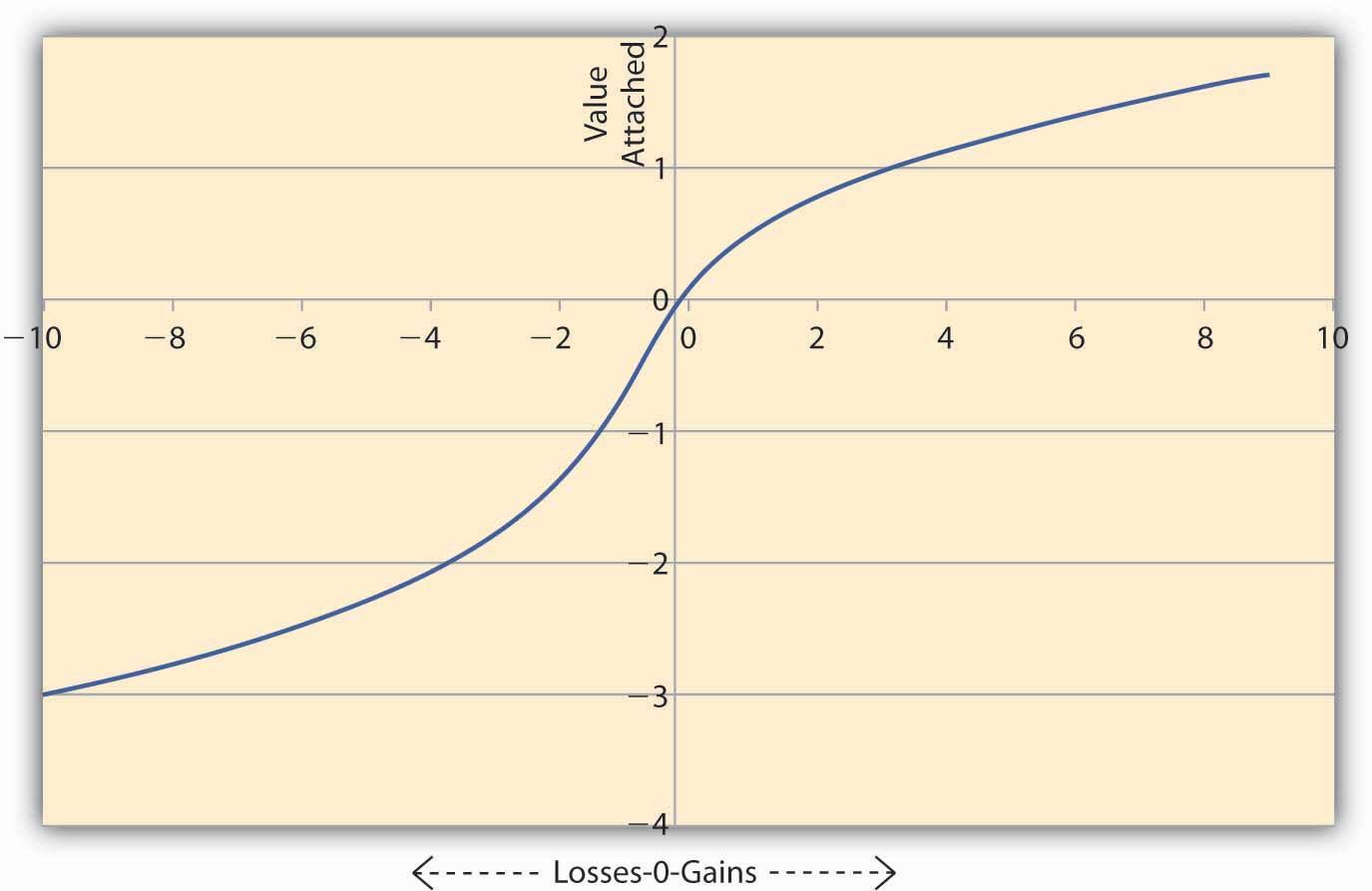
Figure 3.5 "Value Function of Kahneman and Tversky" shows the asymmetric nature of the value function. A loss of $200 causes the individual to feel more value is lost compared to an equivalent gain of $200. To see this notice that on the losses side (the negative x-axis) the graph falls more steeply than the rise in the graph on the gains side (positive x-axis). And this is true regardless of the initial level of wealth the person has initially.
The implications of this type of value function for marketers and sellers are enormous. Note that the value functions are convex in losses. Thus, if $L is lost then say the value lost = Now if there are two consecutive losses of $2 and $3, then the total value lost feels like V (lost) = On the other hand if the losses are combined, then total loss = $5, and the value lost feels like Thus, when losses are combined, the total value lost feels less painful than when the losses are segregated and reported separately.
We can carry out similar analysis on the Kahneman and Tversky function when there is a gain. Note the value function is concave in gains, say, Now if we have two consecutive gains of $2 and $3, then the total value gained feels like V (gain) = On the other hand, if we combine the gains, then total gains = $5, and the value gained feels like Thus, when gains are segregated, the sum of the value of gains turns out to be higher than the value of the sum of gains. So the idea would be to report combined losses, while segregating gains.
Since the individual feels differently about losses and gains, the analysis of the value function tells us that to offset a small loss, we require a larger gain. So small losses can be combined with larger gains, and the individual still feels “happier” since the net effect will be that of a gain. However, if losses are too large, then combining them with small gains would result in a net loss, and the individual would feel that value has been lost. In this case, it’s better to segregate the losses from the gains and report them separately. Such a course of action will provide a consolation to the individual of the type: “At least there are some gains, even if we suffer a big loss.”
Framing effects are not the only reason why people deviate from the behavior predicted by E(U) theory. We discuss some other reasons next, though the list is not exhaustive; a complete study is outside the scope of the text.
-
Overweighting and underweighting of probabilities. Recall that E(U) is the sum of products of two sets of numbers: first, the utility one receives in each state of the world and second, the probabilities with which each state could occur. However, most of the time probabilities are not assigned objectively, but subjectively. For example, before Hurricane Katrina in 2005, individuals in New Orleans would assign a very small probability to flooding of the type experienced in the aftermath of Katrina. However, after the event, the subjective probability estimates of flooding have risen considerably among the same set of individuals.
Humans tend to give more weight to events of the recent past than to look at the entire history. We could attribute such a bias to limited memory, individuals’ myopic view, or just easy availability of more recent information. We call this bias to work with whatever information is easily availability an availability biasTendency to work with whatever information is easily availability.. But people deviate from E(U) theory for more reasons than simply weighting recent past more versus ignoring overall history.
Individuals also react to experience biasTendency to assign more weight to the state of the world that we have experienced and less to others.. Since all of us are shaped somewhat by our own experiences, we tend to assign more weight to the state of the world that we have experienced and less to others. Similarly, we might assign a very low weight to a bad event occurring in our lives, even to the extent of convincing ourselves that such a thing could never happen to us. That is why we see women avoiding mammograms and men colonoscopies. On the other hand, we might attach a higher-than-objective probability to good things happening to us. No matter what the underlying cause is, availability or experience, we know empirically that the probability weights are adjusted subjectively by individuals. Consequently, their observed behavior deviates from E(U) theory.
-
Anchoring bias. Often individuals base their subjective assessments of outcomes based on an initial “guesstimate.” Such a guess may not have any reasonable relationship to the outcomes being studied. In an experimental study reported by Kahneman and Tversky in Science (1974), the authors point this out. The authors call this anchoring biasTendency to base subjective assessments of outcomes on an initial estimate.; it has the effect of biasing the probability estimates of individuals. The experiment they conducted ran as follows:
First, each individual under study had to spin a wheel of fortune with numbers ranging from zero to one hundred. Then, the authors asked the individual if the percent of African nations in the United Nations (UN) was lower or higher than the number on the wheel. Finally, the individuals had to provide an estimate of the percent of African nations in the UN. The authors observed that those who spun a 10 or lower had a median estimate of 25 percent, while those who spun 65 or higher provided a median estimate of 45 percent.
Notice that the number obtained on the wheel had no correlation with the question being asked. It was a randomly generated number. However, it had the effect of making people anchor their answers around the initial number that they had obtained. Kahneman and Tversky also found that even if the payoffs to the subjects were raised to encourage people to provide a correct estimate, the anchoring effect was still evident.
-
Failure to ignore sunk costs. This is the most common reason why we observe departures from E(U) theory. Suppose a person goes to the theater to watch a movie and discovers that he lost $10 on the way. Another person who had bought an online ticket for $10 finds he lost the ticket on the way. The decision problem is: “Should these people spend another $10 to watch the movie?” In experiments conducted suggesting exactly the same choices, respondents’ results show that the second group is more likely to go home without watching the movie, while the first one will overwhelmingly (88 percent) go ahead and watch the movie.
Why do we observe this behavior? The two situations are exactly alike. Each group lost $10. But in a world of mental accounting, the second group has already spent the money on the movie. So this group mentally assumes a cost of $20 for the movie. However, the first group had lost $10 that was not marked toward a specific expense. The second group does not have the “feel” of a lost ticket worth $10 as a sunk costMoney spent that cannot be recovered., which refers to money spent that cannot be recovered. What should matter under E(U) theory is only the value of the movie, which is $10. Whether the ticket or cash was lost is immaterial. Systematic accounting for sunk costs (which economists tell us that we should ignore) causes departures from rational behavior under E(U) theory.
The failure to ignore sunk costs can cause individuals to continue to invest in ventures that are already losing money. Thus, somebody who bought shares at $1,000 that now trade at $500 will continue to hold on to them. They realized that the $1,000 is sunk and thus ignore it. Notice that under rational expectations, what matters is the value of the shares now. Mental accounting tells the shareholders that the value of the shares is still $1,000; the individual does not sell the shares at $500. Eventually, in the economists’ long run, the shareholder may have to sell them for $200 and lose a lot more. People regard such a loss in value as a paper loss versus real loss, and individuals may regard real loss as a greater pain than a paper loss.
By no mean is the list above complete. Other kinds of cognitive biases intervene that can lead to deviating behavior from E(U) theory. But we must notice one thing about E(U) theory versus the value function approach. The E(U) theory is an axiomatic approach to the study of human behavior. If those axioms hold, it can actually predict behavior. On the other hand the value function approach is designed only to describe what actually happens, rather than what should happen.
Key Takeaways
- Students should be able to describe the reasons why observed behavior is different from the predicted behavior under E(U) theory.
- They should also be able to discuss the nature of the value function and how it differs from the utility function.
Discussion Questions
- Describe the Kahneman and Tversky value function. What evidence do they offer to back it up?
- Are shapes other than the ones given by utility functions and value function possible? Provide examples and discuss the implications of the shapes.
- Discuss similarities and dissimilarities between availability bias, experience bias, and failure to ignore sunk costs.?
3.5 Risk Aversion and Price of Hedging Risk
Learning Objectives
- In this section we focus on risk aversion and the price of hedging risk. We discuss the actuarially fair premium (AFP) and the risk premium.
- Students will learn how these principles are applied to pricing of insurance (one mechanism to hedge individual risks) and the decision to purchase insurance.
From now on, we will restrict ourselves to the E(U) theory since we can predict behavior with it. We are interested in the predictions about human behavior, rather than just a description of it.
The risk averter’s utility function (as we had seen earlier in Figure 3.2 "A Utility Function for a Risk-Averse Individual") is concave to the origin. Such a person will never play a lottery at its actuarially fair premium, that is, the expected loss in wealth to the individual. Conversely, such a person will always pay at least an actuarially fair premium to get rid of the entire risk.
Suppose Ty is a student who gets a monthly allowance of $200 (initial wealth W0) from his parents. He might lose $100 on any given day with a probability 0.5 or not lose any amount with 50 percent chance. Consequently, the expected loss (E[L]) to Ty equals 0.5($0) + 0.5($100) = $50. In other words, Ty’s expected final wealth E (FW) = 0.5($200 − $0) + 0.5($200 − $100) = W0 − E(L) = $150. The question is how much Ty would be willing to pay to hedge his expected loss of $50. We will assume that Ty’s utility function is given by —a risk averter’s utility function.
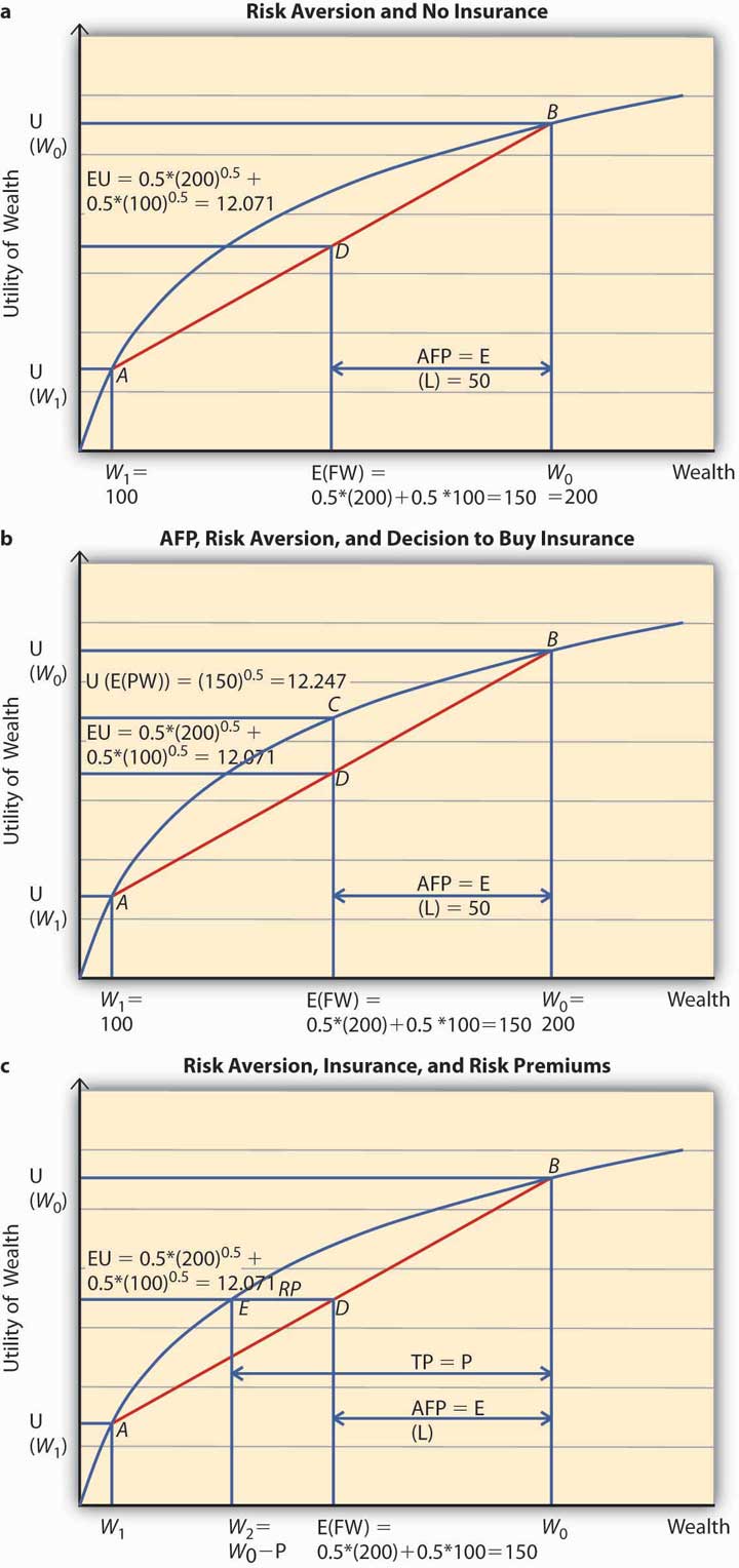
To apply the expected utility theory to answer the question above, we solve the problem in stages. In the first step, we find out Ty’s expected utility when he does not purchase insurance and show it on Figure 3.6 "Risk Aversion" (a). In the second step, we figure out if he will buy insurance at actuarially fair prices and use Figure 3.6 "Risk Aversion" (b) to show it. Finally, we compute Ty’s utility when he pays a premium P to get rid of the risk of a loss. P represents the maximum premium Ty is willing to pay. This is featured in Figure 3.6 "Risk Aversion" (c). At this premium, Ty is exactly indifferent between buying insurance or remaining uninsured. What is P?
Figure 3.6 Risk Aversion
-
Step 1: Expected utility, no insurance.
In case Ty does not buy insurance, he retains all the uncertainty. Thus, he will have an expected final wealth of $150 as calculated above. What is his expected utility?
The expected utility is calculated as a weighted sum of the utilities in the two states, loss and no loss. Therefore, Figure 3.6 "Risk Aversion" (a) shows the point of E(U) for Ty when he does not buy insurance. His expected wealth is given by $150 on the x-axis and expected utility by 12.071 on the y-axis. When we plot this point on the chart, it lies at D, on the chord joining the two points A and B. A and B on the utility curve correspond to the utility levels when a loss is possible (W1 = 100) and no loss (W0 = 200), respectively. In case Ty does not hedge, then his expected utility equals 12.071.
What is the actuarially fair premium for Ty? Note actuarially fair premium (AFP) equals the expected loss = $50. Thus the AFP is the distance between W0 and the E (FW) in Figure 3.6 "Risk Aversion" (a).
-
Step 2: Utility with insurance at AFP.
Now, suppose an insurance company offers insurance to Ty at a $50 premium (AFP). Will Ty buy it? Note that when Ty buys insurance at AFP, and he does not have a loss, his final wealth is $150 (Initial Wealth [$200] − AFP [$50]). In case he does suffer a loss, his final wealth = Initial Wealth ($200) − AFP ($50) − Loss ($100) + Indemnity ($100) = $150. Thus, after the purchase of insurance at AFP, Ty’s final wealth stays at $150 regardless of a loss. That is why Ty has purchased a certain wealth of $150, by paying an AFP of $50. His utility is now given by . This point is represented by C in Figure 3.6 "Risk Aversion" (b). Since C lies strictly above D, Ty will always purchase full insurance at AFP. The noteworthy feature for risk-averse individuals can now be succinctly stated. A risk-averse person will always hedge the risk completely at a cost that equals the expected loss. This cost is the actuarially fair premium (AFP). Alternatively, we can say that a risk-averse person always prefers certainty to uncertainty if uncertainty can be hedged away at its actuarially fair price.
However, the most interesting part is that a risk-averse individual like Ty will pay more than the AFP to get rid of the risk.
-
Step 3: Utility with insurance at a price greater than AFP.
In case the actual premium equals AFP (or expected loss for Ty), it implies the insurance company does not have its own costs/profits. This is an unrealistic scenario. In practice, the premiums must be higher than AFP. The question is how much higher can they be for Ty to still be interested?
To answer this question, we need to answer the question, what is the maximum premium Ty would be willing to pay? The maximum premium P is determined by the point of indifference between no insurance and insurance at price P.
If Ty bears a cost of P, his wealth stands at $200 − P. And this wealth is certain for the same reasons as in step 2. If Ty does not incur a loss, his wealth remains $200 − P. In case he does incur a loss then he gets indemnified by the insurance company. Thus, regardless of outcome his certain wealth is $200 − P.
To compute the point of indifference, we should equate the utility when Ty purchases insurance at P to the expected utility in the no-insurance case. Note E(U) in the no-insurance case in step 1 equals 12.071. After buying insurance at P, Ty’s certain utility is So we solve the equation and get P = $54.29.
Let us see the above calculation on a graph, Figure 3.6 "Risk Aversion" (c). Ty tells himself, “As long as the premium P is such that I am above the E(U) line when I do not purchase insurance, I would be willing to pay it.” So starting from the initial wealth W0, we deduct P, up to the point that the utility of final wealth equals the expected utility given by the point E(U) on the y-axis. This point is given by W2 = W0 − P.
The Total PremiumThe sum of the actuarially fair premium and the risk premium. (TP) = P comprises two parts. The AFP = the distance between initial wealth W0 and E (FW) (= E [L]), and the distance between E (FW) and W2. This distance is called the risk premium (RP, shown as the length ED in Figure 3.6 "Risk Aversion" [c]) and in Ty’s case above, it equals $54.29 − $50 = $4.29.
The premium over and above the AFP that a risk-averse person is willing to pay to get rid of the risk is called the risk premiumThe premium over and above the actuarially fair premium that a risk-averse person is willing to pay to get rid of risk.. Insurance companies are aware of this behavior of risk-averse individuals. However, in the example above, any insurance company that charges a premium greater than $54.29 will not be able to sell insurance to Ty.
Thus, we see that individuals’ risk aversion is a key component in insurance pricing. The greater the degree of risk aversion, the higher the risk premium an individual will be willing to pay. But the insurance price has to be such that the premium charged turns out to be less than or equal to the maximum premium the person is willing to pay. Otherwise, the individual will never buy full insurance.
Thus, risk aversion is a necessary condition for transfer of risks. Since insurance is one mechanism through which a risk-averse person transfers risk, risk aversion is of paramount importance to insurance demand.
The degree of risk aversion is only one aspect that affects insurance prices. Insurance prices also reflect other important components. To study them, we now turn to the role that information plays in the markets: in particular, how information and information asymmetries affect the insurance market.
Key Takeaways
- In this section, students learned that risk aversion is the key to understanding why insurance and other risk hedges exist.
- The student should be able to express the demand for hedging and the conditions under which a risk-averse individual might refuse to transfer risk.
Discussion Questions
- What shape does a risk-averse person’s utility curve take? What role does risk aversion play in market demand for insurance products?
- Distinguish between risk premium and AFP. Show the two on a graph.
- Under what conditions will a risk-averse person refuse an insurance offer?
3.6 Information Asymmetry Problem in Economics
Learning Objective
- Students learn the critical role that information plays in markets. In particular, we discuss two major information economics problems: moral hazard and adverse selection. Students will understand how these two problems affect insurance availability and affordability (prices).
We all know about the used-car market and the market for “lemons.” Akerlof (1970) was the first to analyze how information asymmetryA problem encountered when one party knows more than the other party in the contract. can cause problems in any market. This is a problem encountered when one party knows more than the other party in the contract. In particular, it addresses how information differences between buyers and the sellers (information asymmetry) can cause market failure. These differences are the underlying causes of adverse selectionSituation in which a person with higher risk chooses to hedge the risk, preferably without paying more for the greater risk., a situation under which a person with higher risk chooses to hedge the risk, preferably without paying more for the greater risk. Adverse selection refers to a particular kind of information asymmetry problem, namely, hidden information.
A second kind of information asymmetry lies in the hidden action, wherein one party’s actions are not observable by the counterparty to the contract. Economists study this issue as one of moral hazard.
Adverse Selection
Consider the used-car market. While the sellers of used cars know the quality of their cars, the buyers do not know the exact quality (imagine a world with no blue book information available). From the buyer’s point of view, the car may be a lemon. Under such circumstances, the buyer’s offer price reflects the average quality of the cars in the market.
When sellers approach a market in which average prices are offered, sellers who know that their cars are of better quality do not sell their cars. (This example can be applied to the mortgage and housing crisis in 2008. Sellers who knew that their houses are worth more prefer to hold on to them, instead of lowering the price in order to just make a sale). When they withdraw their cars from market, the average quality of the cars for sale goes down. Buyers’ offer prices get revised downward in response. As a result, the new level of better-quality car sellers withdraws from the market. As this cycle continues, only lemons remain in the market, and the market for used cars fails. As a result of an information asymmetry, the bad-quality product drives away the good-quality ones from the market. This phenomenon is called adverse selection.
It’s easy to demonstrate adverse selection in health insurance. Imagine two individuals, one who is healthy and the other who is not. Both approach an insurance company to buy health insurance policies. Assume for a moment that the two individuals are alike in all respects but their health condition. Insurers can’t observe applicants’ health status; this is private information. If insurers could find no way to figure out the health status, what would it do?
Suppose the insurer’s price schedule reads, “Charge $10 monthly premium to the healthy one, and $25 to the unhealthy one.” If the insurer is asymmetrically informed of the health status of each applicant, it would charge an average premium to each. If insurers charge an average premium, the healthy individual would decide to retain the health risk and remain uninsured. In such a case, the insurance company would be left with only unhealthy policyholders. Note that these less-healthy people would happily purchase insurance, since while their actual cost should be $25 they are getting it for $17.50. In the long run, however, what happens is that the claims from these individuals exceed the amount of premium collected from them. Eventually, the insurance company may become insolvent and go bankrupt. Adverse selection thus causes bankruptcy and market failure. What is the solution to this problem? The easiest is to charge $25 to all individuals regardless of their health status. In a monopolistic marketA market with only one supplier. of only one supplier without competition this might work but not in a competitive market. Even in a close-to-competitive market the effect of adverse selection is to increase prices.
How can one mitigate the extent of adverse selection and its effects? The solution lies in reducing the level of information asymmetry. Thus we find that insurers ask a lot of questions to determine the risk types of individuals. In the used-car market, the buyers do the same. Specialized agencies provide used-car information. Some auto companies certify their cars. And buyers receive warranty offers when they buy used cars.
Insurance agents ask questions and undertake individuals’ risk classification according to risk types. In addition, leaders in the insurance market also developed solutions to adverse selection problems. This comes in the form of risk sharing, which also means partial insurance. Under partial insurance, companies offer products with deductiblesInitial part of the loss absorbed by the person who incurs the loss. (the initial part of the loss absorbed by the person who incurs the loss) and coinsuranceSituation where individuals share in the losses with the insurance companies., where individuals share in the losses with the insurance companies. It has been shown that high-risk individuals prefer full insurance, while low-risk individuals choose partial insurance (high deductibles and coinsurance levels). Insurance companies also offer policies where the premium is adjusted at a later date based on the claim experience of the policyholder during the period.
Moral Hazard
Adverse selection refers to a particular kind of information asymmetry problem, namely, hidden information. A second kind of information asymmetry lies in the hidden action, if actions of one party of the contract are not clear to the other. Economists study these problems under a category called the moral hazard problem.
The simplest way to understand the problem of “observability” (or clarity of action) is to imagine an owner of a store who hires a manager. The store owner may not be available to actually monitor the manager’ actions continuously and at all times, for example, how they behave with customers. This inability to observe actions of the agent (manager) by the principal (owner) falls under the class of problems called the principal-agent problemThe inability of the principal (owner) to observe actions of the agent (manager)..The complete set of principal-agent problems comprises all situations in which the agent maximizes his own utility at the expense of the principal. Such behavior is contrary to the principal-agent relationship that assumes that the agent is acting on behalf of the principal (in principal’s interest). Extension of this problem to the two parties of the insurance contract is straightforward.
Let us say that the insurance company has to decide whether to sell an auto insurance policy to Wonku, who is a risk-averse person with a utility function given by Wonku’s driving record is excellent, so he can claim to be a good risk for the insurance company. However, Wonku can also choose to be either a careful driver or a not-so-careful driver. If he drives with care, he incurs a cost.
To exemplify, let us assume that Wonku drives a car carrying a market value of $10,000. The only other asset he owns is the $3,000 in his checking account. Thus, he has a total initial wealth of $13,000. If he drives carefully, he incurs a cost of $3,000. Assume he faces the following loss distributions when he drives with or without care.
Table 3.3 Loss Distribution
| Drives with Care | Drives without Care | ||
|---|---|---|---|
| Probability | Loss | Probability | Loss |
| 0.25 | 10,000 | 0.75 | 10,000 |
| 0.75 | 0 | 0.25 | 0 |
Table 3.3 "Loss Distribution" shows that when he has an accident, his car is a total loss. The probabilities of “loss” and “no loss” are reversed when he decides to drive without care. The E(L) equals $2,500 in case he drives with care and $7,500 in case he does not. Wonku’s problem has four parts: whether to drive with or without care, (I) when he has no insurance and (II) when he has insurance.
We consider Case I when he carries no insurance. Table 3.4 "Utility Distribution without Insurance" shows the expected utility of driving with and without care. Since care costs $3,000, his initial wealth gets reduced to $10,000 when driving with care. Otherwise, it stays at $13,000. The utility distribution for Wonku is shown in Table 3.4 "Utility Distribution without Insurance".
Table 3.4 Utility Distribution without Insurance
| Drives with Care | Drives without Care | ||
|---|---|---|---|
| Probability | U (Final Wealth) | Probability | U (Final Wealth) |
| 0.25 | 0 | 0.75 | 54.77 |
| 0.75 | 100 | 0.25 | 114.02 |
When he drives with care and has an accident, then his final wealth (FW) and the utility = In case he does not have an accident and drives with care then his final wealth (FW) = (note that the cost of care, $3,000, is still subtracted from the initial wealth) and the utility = Hence, E(U) of driving with care = Let’s go through it in bullets and make sure each case is clarified.
- When Wonku drives without care he does not incur cost of care, so his initial wealth = $13,000. If he is involved in an accident, his final wealth and the utility = Otherwise, his final wealth and the utility = Computing the expected utility the same way as in the paragraph above, we get
- In Case I, when Wonku does not carry insurance, he will drive carefully since his expected utility is higher when he exercises due care. His utility is 75 versus 69.58.
- In Case II we assume that Wonku decides to carry insurance, and claims to the insurance company. He is a careful driver. Let us assume that his insurance policy is priced based on this claim. Assuming the insurance company’s profit and expense loading factor equals 10 percent of AFP (actuarially fair premium), the premium demanded is Wonku needs to decide whether or not to drive with care.
- We analyze the decision based on E(U) as in Case I. The wealth after purchase of insurance equals $10,250. The utility in cases of driving with care or without care is shown in Table 3.5 "Utility Distribution with Insurance" below.
Table 3.5 Utility Distribution with Insurance
| Drives with Care | Drives without Care | ||
|---|---|---|---|
| Probability | U (FW) | Probability | U (FW) |
| 0.25 | 85.15 | 0.75 | 101.24 |
| 0.75 | 85.15 | 0.25 | 101.24 |
Notice that after purchase of insurance, Wonku has eliminated the uncertainty. So if he has an accident, the insurance company indemnifies him with $10,000. Thus, when Wonku has insurance, the following are the possibilities:
-
He is driving with care
- And his car gets totaled, his final wealth = and associated utility =
- And no loss occurs, his final wealth =
So the expected utility for Wonku = 85.15 when he drives with care.
-
He does not drive with care
- And his car gets totaled, his final wealth = and associated utility =
- And no loss occurs, his final wealth = $10,250 and utility = 101.24.
So the expected utility for Wonku = 101.24 when he drives without care after purchasing insurance.
The net result is he switches to driving with no care.
Wonku’s behavior thus changes from driving with care to driving without care after purchasing insurance. Why do we get this result? In this example, the cost of insurance is cheaper than the cost of care. Insurance companies can charge a price greater than the cost of care up to a maximum of what Wonku is willing to pay. However, in the event of asymmetric information, the insurance company will not know the cost of care. Thus, inexpensive insurance distorts the incentives and individuals switch to riskier behavior ex post.
In this moral hazard example, the probabilities of having a loss are affected, not the loss amounts. In practice, both will be affected. At its limit, when moral hazard reaches a point where the intention is to cheat the insurance company, it manifests itself in fraudulent behavior.
How can we solve this problem? An ideal solution would be continuous monitoring, which is prohibitively expensive and may not even be legal for privacy issues. Alternatively, insurance companies try and gather as much information as possible to arrive at an estimate of the cost of care or lack of it. Also, more information leads to an estimate of the likelihood that individuals will switch to riskier behavior afterwards. So questions like marital status/college degree and other personal information might be asked. Insurance companies will undertake a process called risk classification. We discuss this important process later in the text.
So far we have learned how individuals’ risk aversion and information asymmetry explain behavior associated with hedging. But do these reasons also hold when we study why corporations hedge their risks? We provide the answer to this question next.
Key Takeaways
- Students should be able to define information asymmetry problems, in particular moral hazard and adverse selection.
- They must also be able to discuss in detail the effects these phenomena have on insurance prices and risk transfer markets in general.
- Students should spend some effort to understand computations, which are so important if they wish to fully understand the effects that these computations have on actuarial science. Insurance companies make their decisions primarily on the basis of such calculations.
Discussion Questions
- What information asymmetry problems arise in economics? Distinguish between moral hazard and adverse selection. Give an original example of each.
- What effects can information asymmetry have in markets?
- Is risk aversion a necessary condition for moral hazard or adverse selection to exist? Provide reasons.
- What can be done to mitigate the effect of moral hazard and adverse selection in markets/insurance markets?
3.7 Why Corporations Hedge
Learning Objective
- Why should corporations hedge? Financial theory tells us that in a perfect world, corporations are risk neutral. Students can learn in this section the reasons why large companies hedge risk, and, in particular, why they buy insurance.
Financial theory tells us that corporations are risk neutral. This is because only the systematic risk matters, while a particular company can diversify the idiosyncratic riskSystematic risk is the risk that everyone has to share, each according to his/her capacity. Idiosyncratic risk, on the other hand, falls only on a small section of the population. While systematic risk cannot be transferred to anyone outside since it encompasses all agents, idiosyncratic risk can be transferred for a price. That is why idiosyncratic risk is called diversifiable, and systematic is not. The economy-wide recession that unfolded in 2008 is a systematic risk in which everyone is affected. away. If we think about a large company held by a large number of small shareholders like us, then we’d prefer that the company not hedge its risks. In fact, if we wanted to hedge those risks we can do it ourselves. We hold a particular company’s shares because we are looking for those particular risks.
Look back at Figure 3.4 "A Utility Function for a Risk-Neutral Individual". Since firms are risk neutral, their value function is the straight line that appears in the figure. Thus corporations will hedge risk only at their AFP, otherwise they will not. But we know that insurance companies cannot really sell policies at AFP, since they also have to cover their costs and profits. Yet we find that corporations still buy these hedging instruments at greater price than AFP. Therefore, to find a rationale for corporations hedging behavior, we have to move beyond the individual level utility functions of risk aversion.
The following are several reasons for companies hedging behavior:
- Managers hedge because they are undiversified: Small shareholders like us can diversify our risks, but managers cannot. They invest their income from labor as well as their personal assets in the firm. Therefore, while owners (principals) are diversified, managers (agents) are not. Since managers are risk averse and they control the company directly, they hedge.
- Managers want to lower expected bankruptcy costs: If a company goes bankrupt, then bankruptcy supervisors investigate and retain a part of the company’s assets. The wealth gets transferred to third parties and constitutes a loss of assets to the rightful owners. Imagine a fire that destroys the plant. If the company wants to avoid bankruptcy, it might want to rebuild it. If rebuilding is financed through debt financing, the cost of debt is going to be very high because the company may not have any collateral to offer. In this case, having fire insurance can serve as collateral as well as compensate the firm when it suffers a loss due to fire.
- Risk bearers may be in a better position to bear the risk: Companies may not be diversified, in terms of either product or geography. They may not have access to broader capital markets because of small size. Companies may transfer risk to better risk bearers that are diversified and have better and broader access to capital markets.
- Hedging can increase debt capacity: Financial theory tells us about an optimal capital structureA company’s optimal mix of debt and equity financing. for every company. This means that each company has an optimal mix of debt and equity financing. The amount of debt determines the financial risk to a company. With hedging, the firm can transfer the risk outside the firm. With lower risk, the firm can undertake a greater amount of debt, thus changing the optimal capital structure.
- Lowering of tax liability: Since insurance premiums are tax deductible for some corporate insurance policies, companies can lower the expected taxes by purchasing insurance.
- Other reasons: We can cite some other reasons why corporations hedge. Regulated companies are found to hedge more than unregulated ones, probably because law limits the level of risk taking. Laws might require companies to purchase some insurance mandatorily. For example, firms might need aircraft liability insurance, third-party coverage for autos, and workers compensation. Firms may also purchase insurance to signal credit worthiness (e.g., construction coverage for commercial builders). Thus, the decision to hedge can reduce certain kinds of information asymmetry problems as well.
We know that corporations hedge their risks, either through insurance or through other financial contracts. Firms can use forwards and futures, other derivatives, and option contracts to hedge their risk. The latter are not pure hedges and firms can use them to take on more risks instead of transferring them outside the firm. Forwards and futures, derivatives, and option contracts present the firm with double-edged swords. Still, because of their complex nature, corporations are in a better position to use it than the individuals who mostly use insurance contracts to transfer their risk.
Key Takeaways
- The student should be able to able to distinguish between individual demand and corporate demand for risk hedging.
- The student should be able to understand and express reasons for corporate hedging.
Discussion Questions
- Which risks matter for corporations: systematic or idiosyncratic? Why?
- Why can’t the rationale of hedging used to explain risk transfer at individual level be applied to companies?
- Describe the reasons why companies hedge their risks. Provide examples.
- What is an optimal capital structure?
3.8 Review and Practice
- What is risk? How is it philosophically different from uncertainty?
- What is asymmetric information? Explain how it leads to market failures in an otherwise perfectly competitive market.
- Explain the difference between moral hazard and adverse selection. Can one exist without the other?
- What externalities are caused in the insurance market by moral hazard and adverse selection? How are they overcome in practice?
- Do risk-averse individuals outnumber risk-seeking ones? Give an intuitive explanation.
- Provide examples that appear to violate expected utility theory and risk aversion.
- Give two examples that tell how the framing of alternatives affects peoples’ choices under uncertainty.
- Suppose you are a personal financial planner managing the portfolio of your mother. In a recession like the one in 2008, there are enormous losses and very few gains to the assets in the portfolio you suggested to your mother. Given the material covered in this chapter, suggest a few marketing strategies to minimize the pain of bad news to your mother.
- Distinguish, through examples, between sunk cost, availability bias, and anchoring effect as reasons for departure from the expected utility paradigm.
- Suppose Yuan Yuan wants to purchase a house for investment purposes. She will rent it out after buying it. She has two choices. Either buy it in an average location where the lifetime rent from the property will be $700,000 with certainty or buy it in an upscale location. However, in the upscale neighborhood there is a 60 percent chance that the lifetime income will equal $1 million and 40 percent chance it will equal only $250,000. If she has a utility function that equals , Where would she prefer to buy the house?
- What is the expected value when a six-sided fair die is tossed?
- Suppose Yijia’s utility function is given by LN(W) and her initial wealth is $500,000. If there is a 0.01 percent chance that a liability lawsuit will reduce her wealth to $50,000, how much premium will she be willing to pay to get rid of the risk?
- Your professor of economics tells you, “The additional benefit that a person derives from a given increase of his stock of a thing decreases with every increase in the stock he already has.” What type of risk attitude does such a person have?
- Ms. Frangipani prefers Pepsi to Coke on a rainy day; Coke to Pepsi on a sunny one. On one sunny day at the CNN center in Atlanta, when faced with a choice between Pepsi, Coke, and Lipton iced tea, she decides to have a Pepsi. Should the presence of iced teas in the basket of choices affect her decision? Does she violate principles of utility maximization? If yes, which assumptions does she violate? If not, then argue how her choices are consistent with the utility theory.
- Explain why a risk-averse person will purchase insurance for the following scenario: Lose $20,000 with 5 percent chance or lose $0 with 95 percent probability. The premium for the policy is $1,000.
-
Imagine that you face the following pair of concurrent decisions. First examine both decisions, then indicate the options you prefer:
Decision (i) Choose between
- a sure gain of $240,
- 25 percent chance to gain $1,000, and 75 percent chance to gain nothing.
Decision (ii) Choose between:
- a sure loss of $750,
- 75 percent chance to lose $1,000 and 25 percent chance to lose nothing.
Indicate which option you would choose in each of the decisions and why.This problem has been adopted from D. Kahneman and D. Lovallo, “Timid Choices and Bold Forecasts: A Cognitive Perspective on Risk Taking,” Management Science 39, no. 1 (1993): 17–31.
-
Consider the following two lotteries:
- Gain of $100 with probability 0.75; no gain ($0 gain) with probability 0.25
- Gain of $1,000 with probability 0.05; no gain ($0 gain) with probability 0.95
Which of these lotteries will you prefer to play?
Now, assume somebody promises you sure sums of money so as to induce you to not play the lotteries. What is the sure sum of money you will be willing to accept in case of each lottery: a or b? Is your decision “rational”?
-
Partial insurance:Challenging problem. This problem is designed to illustrate why partial insurance (i.e., a policy that includes deductibles and coinsurance) may be optimal for a risk-averse individual.
Suppose Marco has an initial wealth of $1,000 and a utility function given by . He faces the following loss distribution:
Prob Loss 0.9 0 0.1 500 - If the price per unit of insurance is $0.10 per dollar of loss, show that Marco will purchase full insurance (i.e., quantity for which insurance is purchased = $500).
- If the price per unit of insurance is $0.11 per dollar of loss, show that Marco will purchase less than full insurance (i.e., quantity for which insurance is purchased is less than $500). Hint: Compute E(U) for full $500 loss and also for an amount less than $500. See that when he insures strictly less than $500, the EU is higher.
- Otgo has a current wealth of $500 and a lottery ticket that pays $50 with probability 0.25; otherwise, it pays nothing. If her utility function is given by , what is the minimum amount she is willing to sell the ticket for?
-
Suppose a coin is tossed twice in a row. The payoffs associated with the outcomes are
Outcome Win (+) or loss (−) H-H +15 H-T +9 T-H −6 T-T −12 If the coin is unbiased, what is the fair value of the gamble?
-
If you apply the principle of framing to put a favorable spin to events in your life, how would you value the following gains or losses?
- A win of $100 followed by a loss of $20
- A win of $20 followed by a loss of $100
- A win of $50 followed by a win of $60
- A loss of $50 followed by a win of $60
- Explain in detail what happens to an insurer that charges the same premium to teenage drivers as it does to the rest of its customers.
- Corporations are risk neutral, yet they hedge. Why?