This is “Indifference Curve Analysis: An Alternative Approach to Understanding Consumer Choice”, section 7.3 from the book Economics Principles (v. 1.0). For details on it (including licensing), click here.
For more information on the source of this book, or why it is available for free, please see the project's home page. You can browse or download additional books there. To download a .zip file containing this book to use offline, simply click here.


7.3 Indifference Curve Analysis: An Alternative Approach to Understanding Consumer Choice
Learning Objectives
- Explain utility maximization using the concepts of indifference curves and budget lines.
- Explain the notion of the marginal rate of substitution and how it relates to the utility-maximizing solution.
- Derive a demand curve from an indifference map.
Economists typically use a different set of tools than those presented in the chapter up to this point to analyze consumer choices. While somewhat more complex, the tools presented in this section give us a powerful framework for assessing consumer choices.
We will begin our analysis with an algebraic and graphical presentation of the budget constraint. We will then examine a new concept that allows us to draw a map of a consumer’s preferences. Then we can draw some conclusions about the choices a utility-maximizing consumer could be expected to make.
The Budget Line
As we have already seen, a consumer’s choices are limited by the budget available. Total spending for goods and services can fall short of the budget constraint but may not exceed it.
Algebraically, we can write the budget constraint for two goods X and Y as:
Equation 7.7
where PX and PY are the prices of goods X and Y and QX and QY are the quantities of goods X and Y chosen. The total income available to spend on the two goods is B, the consumer’s budget. Equation 7.7 states that total expenditures on goods X and Y (the left-hand side of the equation) cannot exceed B.
Suppose a college student, Janet Bain, enjoys skiing and horseback riding. A day spent pursuing either activity costs $50. Suppose she has $250 available to spend on these two activities each semester. Ms. Bain’s budget constraint is illustrated in Figure 7.9 "The Budget Line".
For a consumer who buys only two goods, the budget constraint can be shown with a budget line. A budget lineGraphically shows the combinations of two goods a consumer can buy with a given budget. shows graphically the combinations of two goods a consumer can buy with a given budget.
The budget line shows all the combinations of skiing and horseback riding Ms. Bain can purchase with her budget of $250. She could also spend less than $250, purchasing combinations that lie below and to the left of the budget line in Figure 7.9 "The Budget Line". Combinations above and to the right of the budget line are beyond the reach of her budget.
Figure 7.9 The Budget Line
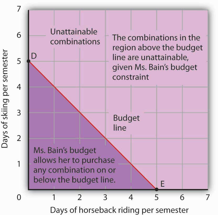
The budget line shows combinations of the skiing and horseback riding Janet Bain could consume if the price of each activity is $50 and she has $250 available for them each semester. The slope of this budget line is −1, the negative of the price of horseback riding divided by the price of skiing.
The vertical intercept of the budget line (point D) is given by the number of days of skiing per month that Ms. Bain could enjoy, if she devoted all of her budget to skiing and none to horseback riding. She has $250, and the price of a day of skiing is $50. If she spent the entire amount on skiing, she could ski 5 days per semester. She would be meeting her budget constraint, since:
The horizontal intercept of the budget line (point E) is the number of days she could spend horseback riding if she devoted her $250 entirely to that sport. She could purchase 5 days of either skiing or horseback riding per semester. Again, this is within her budget constraint, since:
Because the budget line is linear, we can compute its slope between any two points. Between points D and E the vertical change is −5 days of skiing; the horizontal change is 5 days of horseback riding. The slope is thus . More generally, we find the slope of the budget line by finding the vertical and horizontal intercepts and then computing the slope between those two points. The vertical intercept of the budget line is found by dividing Ms. Bain’s budget, B, by the price of skiing, the good on the vertical axis (PS). The horizontal intercept is found by dividing B by the price of horseback riding, the good on the horizontal axis (PH). The slope is thus:
Equation 7.8
Simplifying this equation, we obtain
Equation 7.9
After canceling, Equation 7.9 shows that the slope of a budget line is the negative of the price of the good on the horizontal axis divided by the price of the good on the vertical axis.
Heads Up!
It is easy to go awry on the issue of the slope of the budget line: It is the negative of the price of the good on the horizontal axis divided by the price of the good on the vertical axis. But does not slope equal the change in the vertical axis divided by the change in the horizontal axis? The answer, of course, is that the definition of slope has not changed. Notice that Equation 7.8 gives the vertical change divided by the horizontal change between two points. We then manipulated Equation 7.8 a bit to get to Equation 7.9 and found that slope also equaled the negative of the price of the good on the horizontal axis divided by the price of the good on the vertical axis. Price is not the variable that is shown on the two axes. The axes show the quantities of the two goods.
Indifference Curves
Suppose Ms. Bain spends 2 days skiing and 3 days horseback riding per semester. She will derive some level of total utility from that combination of the two activities. There are other combinations of the two activities that would yield the same level of total utility. Combinations of two goods that yield equal levels of utility are shown on an indifference curveGraph that shows combinations of two goods that yield equal levels of utility..Limiting the situation to two goods allows us to show the problem graphically. By stating the problem of utility maximization with equations, we could extend the analysis to any number of goods and services. Because all points along an indifference curve generate the same level of utility, economists say that a consumer is indifferent between them.
Figure 7.10 "An Indifference Curve" shows an indifference curve for combinations of skiing and horseback riding that yield the same level of total utility. Point X marks Ms. Bain’s initial combination of 2 days skiing and 3 days horseback riding per semester. The indifference curve shows that she could obtain the same level of utility by moving to point W, skiing for 7 days and going horseback riding for 1 day. She could also get the same level of utility at point Y, skiing just 1 day and spending 5 days horseback riding. Ms. Bain is indifferent among combinations W, X, and Y. We assume that the two goods are divisible, so she is indifferent between any two points along an indifference curve.
Figure 7.10 An Indifference Curve
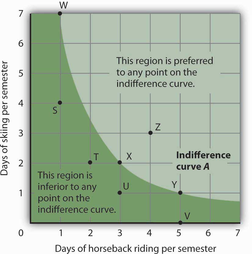
The indifference curve A shown here gives combinations of skiing and horseback riding that produce the same level of utility. Janet Bain is thus indifferent to which point on the curve she selects. Any point below and to the left of the indifference curve would produce a lower level of utility; any point above and to the right of the indifference curve would produce a higher level of utility.
Now look at point T in Figure 7.10 "An Indifference Curve". It has the same amount of skiing as point X, but fewer days are spent horseback riding. Ms. Bain would thus prefer point X to point T. Similarly, she prefers X to U. What about a choice between the combinations at point W and point T? Because combinations X and W are equally satisfactory, and because Ms. Bain prefers X to T, she must prefer W to T. In general, any combination of two goods that lies below and to the left of an indifference curve for those goods yields less utility than any combination on the indifference curve. Such combinations are inferior to combinations on the indifference curve.
Point Z, with 3 days of skiing and 4 days of horseback riding, provides more of both activities than point X; Z therefore yields a higher level of utility. It is also superior to point W. In general, any combination that lies above and to the right of an indifference curve is preferred to any point on the indifference curve.
We can draw an indifference curve through any combination of two goods. Figure 7.11 "Indifference Curves" shows indifference curves drawn through each of the points we have discussed. Indifference curve A from Figure 7.10 "An Indifference Curve" is inferior to indifference curve B. Ms. Bain prefers all the combinations on indifference curve B to those on curve A, and she regards each of the combinations on indifference curve C as inferior to those on curves A and B.
Although only three indifference curves are shown in Figure 7.11 "Indifference Curves", in principle an infinite number could be drawn. The collection of indifference curves for a consumer constitutes a kind of map illustrating a consumer’s preferences. Different consumers will have different maps. We have good reason to expect the indifference curves for all consumers to have the same basic shape as those shown here: They slope downward, and they become less steep as we travel down and to the right along them.
Figure 7.11 Indifference Curves
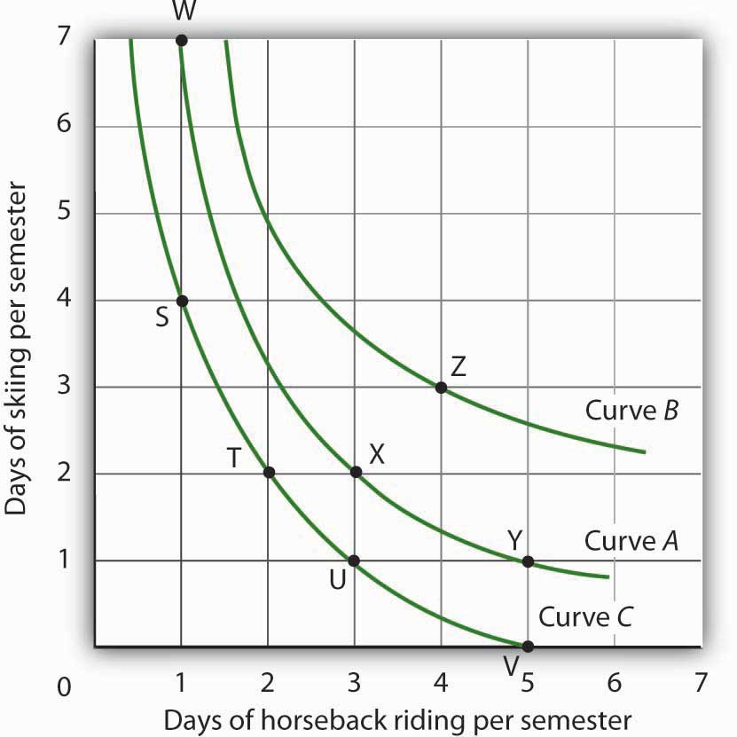
Each indifference curve suggests combinations among which the consumer is indifferent. Curves that are higher and to the right are preferred to those that are lower and to the left. Here, indifference curve B is preferred to curve A, which is preferred to curve C.
The slope of an indifference curve shows the rate at which two goods can be exchanged without affecting the consumer’s utility. Figure 7.12 "The Marginal Rate of Substitution" shows indifference curve C from Figure 7.11 "Indifference Curves". Suppose Ms. Bain is at point S, consuming 4 days of skiing and 1 day of horseback riding per semester. Suppose she spends another day horseback riding. This additional day of horseback riding does not affect her utility if she gives up 2 days of skiing, moving to point T. She is thus willing to give up 2 days of skiing for a second day of horseback riding. The curve shows, however, that she would be willing to give up at most 1 day of skiing to obtain a third day of horseback riding (shown by point U).
Figure 7.12 The Marginal Rate of Substitution
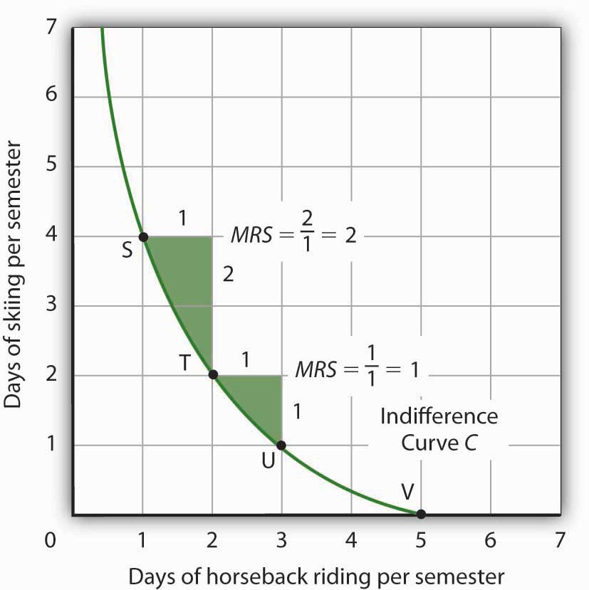
The marginal rate of substitution is equal to the absolute value of the slope of an indifference curve. It is the maximum amount of one good a consumer is willing to give up to obtain an additional unit of another. Here, it is the number of days of skiing Janet Bain would be willing to give up to obtain an additional day of horseback riding. Notice that the marginal rate of substitution (MRS) declines as she consumes more and more days of horseback riding.
The maximum amount of one good a consumer would be willing to give up in order to obtain an additional unit of another is called the marginal rate of substitution (MRS)The maximum amount of one good a consumer would be willing to give up in order to obtain an additional unit of another., which is equal to the absolute value of the slope of the indifference curve between two points. Figure 7.12 "The Marginal Rate of Substitution" shows that as Ms. Bain devotes more and more time to horseback riding, the rate at which she is willing to give up days of skiing for additional days of horseback riding—her marginal rate of substitution—diminishes.
The Utility-Maximizing Solution
We assume that each consumer seeks the highest indifference curve possible. The budget line gives the combinations of two goods that the consumer can purchase with a given budget. Utility maximization is therefore a matter of selecting a combination of two goods that satisfies two conditions:
- The point at which utility is maximized must be within the attainable region defined by the budget line.
- The point at which utility is maximized must be on the highest indifference curve consistent with condition 1.
Figure 7.13 "The Utility-Maximizing Solution" combines Janet Bain’s budget line from Figure 7.9 "The Budget Line" with her indifference curves from Figure 7.11 "Indifference Curves". Our two conditions for utility maximization are satisfied at point X, where she skis 2 days per semester and spends 3 days horseback riding.
Figure 7.13 The Utility-Maximizing Solution
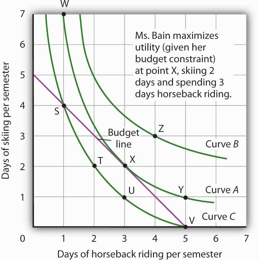
Combining Janet Bain’s budget line and indifference curves from Figure 7.9 "The Budget Line" and Figure 7.11 "Indifference Curves", we find a point that (1) satisfies the budget constraint and (2) is on the highest indifference curve possible. That occurs for Ms. Bain at point X.
The highest indifference curve possible for a given budget line is tangent to the line; the indifference curve and budget line have the same slope at that point. The absolute value of the slope of the indifference curve shows the MRS between two goods. The absolute value of the slope of the budget line gives the price ratio between the two goods; it is the rate at which one good exchanges for another in the market. At the point of utility maximization, then, the rate at which the consumer is willing to exchange one good for another equals the rate at which the goods can be exchanged in the market. For any two goods X and Y, with good X on the horizontal axis and good Y on the vertical axis,
Equation 7.10
Utility Maximization and the Marginal Decision Rule
How does the achievement of The Utility Maximizing Solution in Figure 7.13 "The Utility-Maximizing Solution" correspond to the marginal decision rule? That rule says that additional units of an activity should be pursued, if the marginal benefit of the activity exceeds the marginal cost. The observation of that rule would lead a consumer to the highest indifference curve possible for a given budget.
Suppose Ms. Bain has chosen a combination of skiing and horseback riding at point S in Figure 7.14 "Applying the Marginal Decision Rule". She is now on indifference curve C. She is also on her budget line; she is spending all of the budget, $250, available for the purchase of the two goods.
Figure 7.14 Applying the Marginal Decision Rule
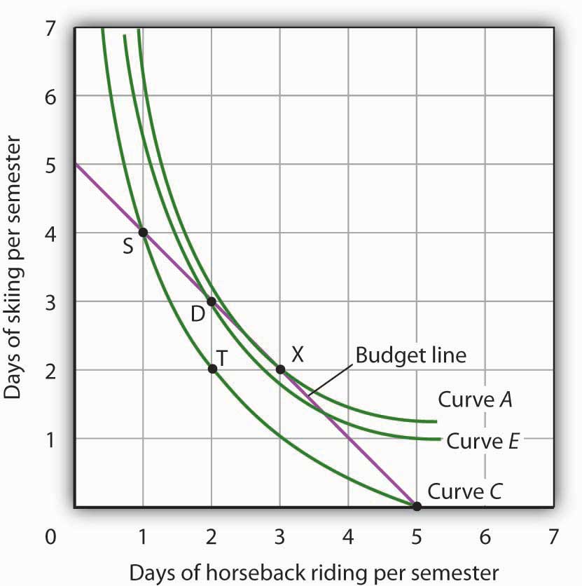
Suppose Ms. Bain is initially at point S. She is spending all of her budget, but she is not maximizing utility. Because her marginal rate of substitution exceeds the rate at which the market asks her to give up skiing for horseback riding, she can increase her satisfaction by moving to point D. Now she is on a higher indifference curve, E. She will continue exchanging skiing for horseback riding until she reaches point X, at which she is on curve A, the highest indifference curve possible.
An exchange of two days of skiing for one day of horseback riding would leave her at point T, and she would be as well off as she is at point S. Her marginal rate of substitution between points S and T is 2; her indifference curve is steeper than the budget line at point S. The fact that her indifference curve is steeper than her budget line tells us that the rate at which she is willing to exchange the two goods differs from the rate the market asks. She would be willing to give up as many as 2 days of skiing to gain an extra day of horseback riding; the market demands that she give up only one. The marginal decision rule says that if an additional unit of an activity yields greater benefit than its cost, it should be pursued. If the benefit to Ms. Bain of one more day of horseback riding equals the benefit of 2 days of skiing, yet she can get it by giving up only 1 day of skiing, then the benefit of that extra day of horseback riding is clearly greater than the cost.
Because the market asks that she give up less than she is willing to give up for an additional day of horseback riding, she will make the exchange. Beginning at point S, she will exchange a day of skiing for a day of horseback riding. That moves her along her budget line to point D. Recall that we can draw an indifference curve through any point; she is now on indifference curve E. It is above and to the right of indifference curve C, so Ms. Bain is clearly better off. And that should come as no surprise. When she was at point S, she was willing to give up 2 days of skiing to get an extra day of horseback riding. The market asked her to give up only one; she got her extra day of riding at a bargain! Her move along her budget line from point S to point D suggests a very important principle. If a consumer’s indifference curve intersects the budget line, then it will always be possible for the consumer to make exchanges along the budget line that move to a higher indifference curve. Ms. Bain’s new indifference curve at point D also intersects her budget line; she’s still willing to give up more skiing than the market asks for additional riding. She will make another exchange and move along her budget line to point X, at which she attains the highest indifference curve possible with her budget. Point X is on indifference curve A, which is tangent to the budget line.
Having reached point X, Ms. Bain clearly would not give up still more days of skiing for additional days of riding. Beyond point X, her indifference curve is flatter than the budget line—her marginal rate of substitution is less than the absolute value of the slope of the budget line. That means that the rate at which she would be willing to exchange skiing for horseback riding is less than the market asks. She cannot make herself better off than she is at point X by further rearranging her consumption. Point X, where the rate at which she is willing to exchange one good for another equals the rate the market asks, gives her the maximum utility possible.
Utility Maximization and Demand
Figure 7.14 "Applying the Marginal Decision Rule" showed Janet Bain’s utility-maximizing solution for skiing and horseback riding. She achieved it by selecting a point at which an indifference curve was tangent to her budget line. A change in the price of one of the goods, however, will shift her budget line. By observing what happens to the quantity of the good demanded, we can derive Ms. Bain’s demand curve.
Panel (a) of Figure 7.15 "Utility Maximization and Demand" shows the original solution at point X, where Ms. Bain has $250 to spend and the price of a day of either skiing or horseback riding is $50. Now suppose the price of horseback riding falls by half, to $25. That changes the horizontal intercept of the budget line; if she spends all of her money on horseback riding, she can now ride 10 days per semester. Another way to think about the new budget line is to remember that its slope is equal to the negative of the price of the good on the horizontal axis divided by the price of the good on the vertical axis. When the price of horseback riding (the good on the horizontal axis) goes down, the budget line becomes flatter. Ms. Bain picks a new utility-maximizing solution at point Z.
Figure 7.15 Utility Maximization and Demand
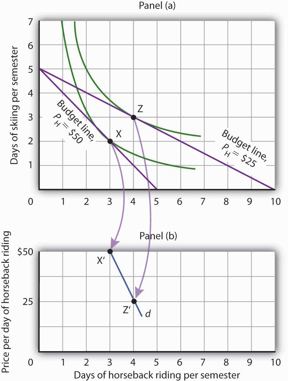
By observing a consumer’s response to a change in price, we can derive the consumer’s demand curve for a good. Panel (a) shows that at a price for horseback riding of $50 per day, Janet Bain chooses to spend 3 days horseback riding per semester. Panel (b) shows that a reduction in the price to $25 increases her quantity demanded to 4 days per semester. Points X and Z, at which Ms. Bain maximizes utility at horseback riding prices of $50 and $25, respectively, become points X′ and Z′ on her demand curve, d, for horseback riding in Panel (b).
The solution at Z involves an increase in the number of days Ms. Bain spends horseback riding. Notice that only the price of horseback riding has changed; all other features of the utility-maximizing solution remain the same. Ms. Bain’s budget and the price of skiing are unchanged; this is reflected in the fact that the vertical intercept of the budget line remains fixed. Ms. Bain’s preferences are unchanged; they are reflected by her indifference curves. Because all other factors in the solution are unchanged, we can determine two points on Ms. Bain’s demand curve for horseback riding from her indifference curve diagram. At a price of $50, she maximized utility at point X, spending 3 days horseback riding per semester. When the price falls to $25, she maximizes utility at point Z, riding 4 days per semester. Those points are plotted as points X′ and Z′ on her demand curve for horseback riding in Panel (b) of Figure 7.15 "Utility Maximization and Demand".
Key Takeaways
- A budget line shows combinations of two goods a consumer is able to consume, given a budget constraint.
- An indifference curve shows combinations of two goods that yield equal satisfaction.
- To maximize utility, a consumer chooses a combination of two goods at which an indifference curve is tangent to the budget line.
- At the utility-maximizing solution, the consumer’s marginal rate of substitution (the absolute value of the slope of the indifference curve) is equal to the price ratio of the two goods.
- We can derive a demand curve from an indifference map by observing the quantity of the good consumed at different prices.
Try It!
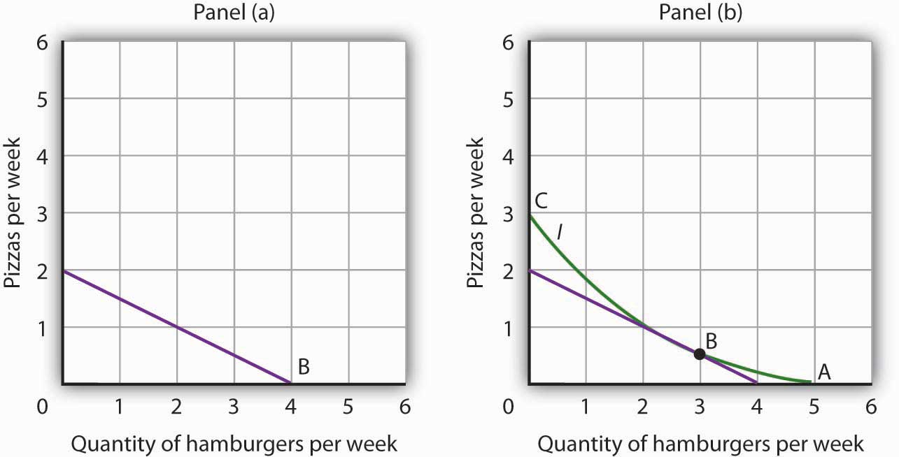
- Suppose a consumer has a budget for fast-food items of $20 per week and spends this money on two goods, hamburgers and pizzas. Suppose hamburgers cost $5 each and pizzas cost $10. Put the quantity of hamburgers purchased per week on the horizontal axis and the quantity of pizzas purchased per week on the vertical axis. Draw the budget line. What is its slope?
-
Suppose the consumer in part (a) is indifferent among the combinations of hamburgers and pizzas shown. In the grid you used to draw the budget lines, draw an indifference curve passing through the combinations shown, and label the corresponding points A, B, and C. Label this curve I.
Combination Hamburgers/week Pizzas/week A 5 0 B 3 ½ C 0 3 - The budget line is tangent to indifference curve I at B. Explain the meaning of this tangency.
Case in Point: Preferences Prevail in P.O.W. Camps
Figure 7.16
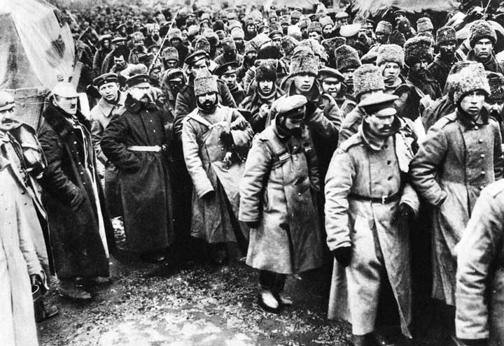
© 2010 Jupiterimages Corporation
Economist R. A. Radford spent time in prisoner of war (P.O.W.) camps in Italy and Germany during World War II. He put this unpleasant experience to good use by testing a number of economic theories there. Relevant to this chapter, he consistently observed utility-maximizing behavior.
In the P.O.W. camps where he stayed, prisoners received rations, provided by their captors and the Red Cross, including tinned milk, tinned beef, jam, butter, biscuits, chocolate, tea, coffee, cigarettes, and other items. While all prisoners received approximately equal official rations (though some did manage to receive private care packages as well), their marginal rates of substitution between goods in the ration packages varied. To increase utility, prisoners began to engage in trade.
Prices of goods tended to be quoted in terms of cigarettes. Some camps had better organized markets than others but, in general, even though prisoners of each nationality were housed separately, so long as they could wander from bungalow to bungalow, the “cigarette” prices of goods were equal across bungalows. Trade allowed the prisoners to maximize their utility.
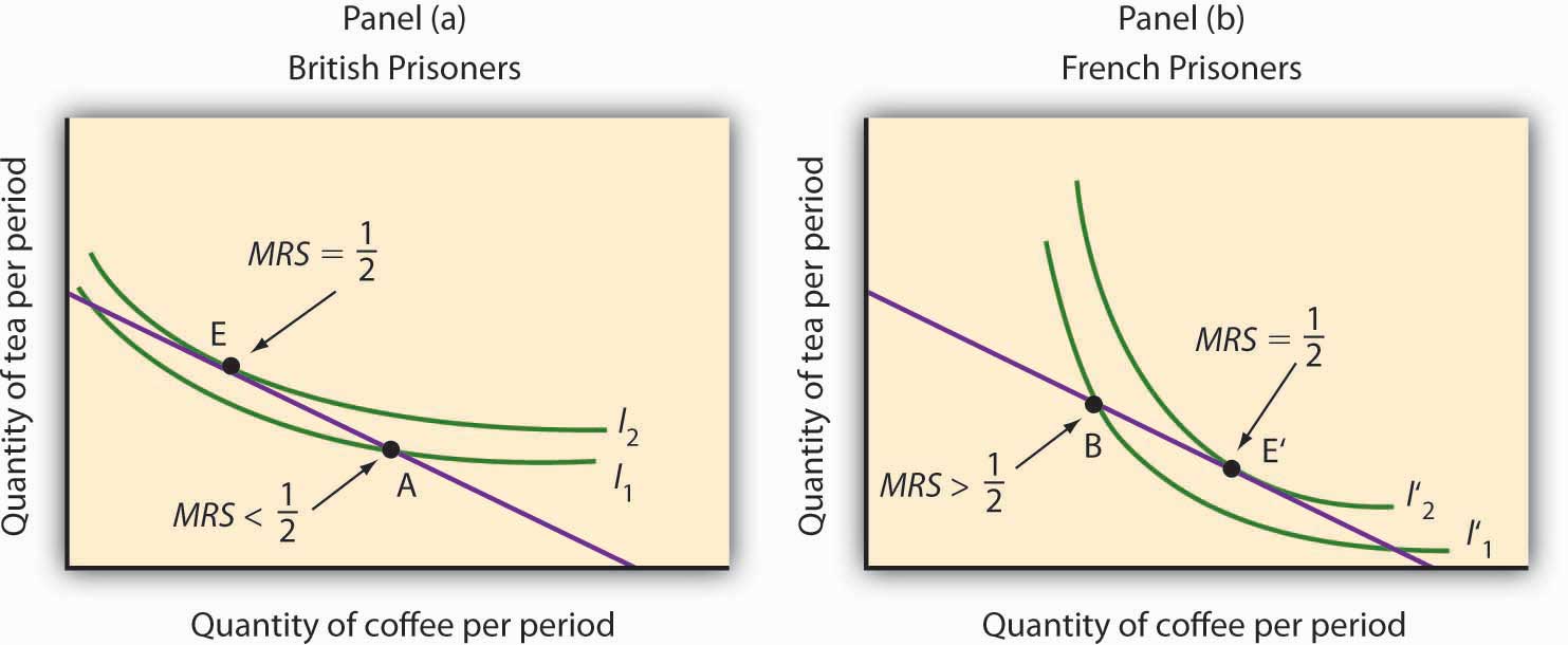
Consider coffee and tea. Panel (a) shows the indifference curves and budget line for typical British prisoners and Panel (b) shows the indifference curves and budget line for typical French prisoners. Suppose the price of an ounce of tea is 2 cigarettes and the price of an ounce of coffee is 1 cigarette. The slopes of the budget lines in each panel are identical; all prisoners faced the same prices. The price ratio is 1/2.
Suppose the ration packages given to all prisoners contained the same amounts of both coffee and tea. But notice that for typical British prisoners, given indifference curves which reflect their general preference for tea, the MRS at the initial allocation (point A) is less than the price ratio. For French prisoners, the MRS is greater than the price ratio (point B). By trading, both British and French prisoners can move to higher indifference curves. For the British prisoners, the utility-maximizing solution is at point E, with more tea and little coffee. For the French prisoners the utility-maximizing solution is at point E′, with more coffee and less tea. In equilibrium, both British and French prisoners consumed tea and coffee so that their MRS’s equal 1/2, the price ratio in the market.
Figure 7.17
Source: R. A. Radford, “The Economic Organisation of a P.O.W. Camp,” Economica 12 (November 1945): 189–201; and Jack Hirshleifer, Price Theory and Applications (Englewood Cliffs, NJ: Prentice Hall, 1976): 85–86.
Answers to Try It! Problems
- The budget line is shown in Panel (a). Its slope is −$5/$10 = −0.5.
- Panel (b) shows indifference curve I. The points A, B, and C on I have been labeled.
-
The tangency point at B shows the combinations of hamburgers and pizza that maximize the consumer’s utility, given the budget constraint. At the point of tangency, the marginal rate of substitution (MRS) between the two goods is equal to the ratio of prices of the two goods. This means that the rate at which the consumer is willing to exchange one good for another equals the rate at which the goods can be exchanged in the market.
Figure 7.18