This is “Chi-Square One-Sample Goodness-of-Fit Tests”, section 11.2 from the book Beginning Statistics (v. 1.0). For details on it (including licensing), click here.
For more information on the source of this book, or why it is available for free, please see the project's home page. You can browse or download additional books there. To download a .zip file containing this book to use offline, simply click here.


11.2 Chi-Square One-Sample Goodness-of-Fit Tests
Learning Objective
- To understand how to use a chi-square test to judge whether a sample fits a particular population well.
Suppose we wish to determine if an ordinary-looking six-sided die is fair, or balanced, meaning that every face has probability 1/6 of landing on top when the die is tossed. We could toss the die dozens, maybe hundreds, of times and compare the actual number of times each face landed on top to the expected number, which would be 1/6 of the total number of tosses. We wouldn’t expect each number to be exactly 1/6 of the total, but it should be close. To be specific, suppose the die is tossed n = 60 times with the results summarized in Table 11.8 "Die Contingency Table". For ease of reference we add a column of expected frequencies, which in this simple example is simply a column of 10s. The result is shown as Table 11.9 "Updated Die Contingency Table". In analogy with the previous section we call this an “updated” table. A measure of how much the data deviate from what we would expect to see if the die really were fair is the sum of the squares of the differences between the observed frequency O and the expected frequency E in each row, or, standardizing by dividing each square by the expected number, the sum If we formulate the investigation as a test of hypotheses, the test is
Table 11.8 Die Contingency Table
| Die Value | Assumed Distribution | Observed Frequency |
|---|---|---|
| 1 | 1/6 | 9 |
| 2 | 1/6 | 15 |
| 3 | 1/6 | 9 |
| 4 | 1/6 | 8 |
| 5 | 1/6 | 6 |
| 6 | 1/6 | 13 |
Table 11.9 Updated Die Contingency Table
| Die Value | Assumed Distribution | Observed Freq. | Expected Freq. |
|---|---|---|---|
| 1 | 1/6 | 9 | 10 |
| 2 | 1/6 | 15 | 10 |
| 3 | 1/6 | 9 | 10 |
| 4 | 1/6 | 8 | 10 |
| 5 | 1/6 | 6 | 10 |
| 6 | 1/6 | 13 | 10 |
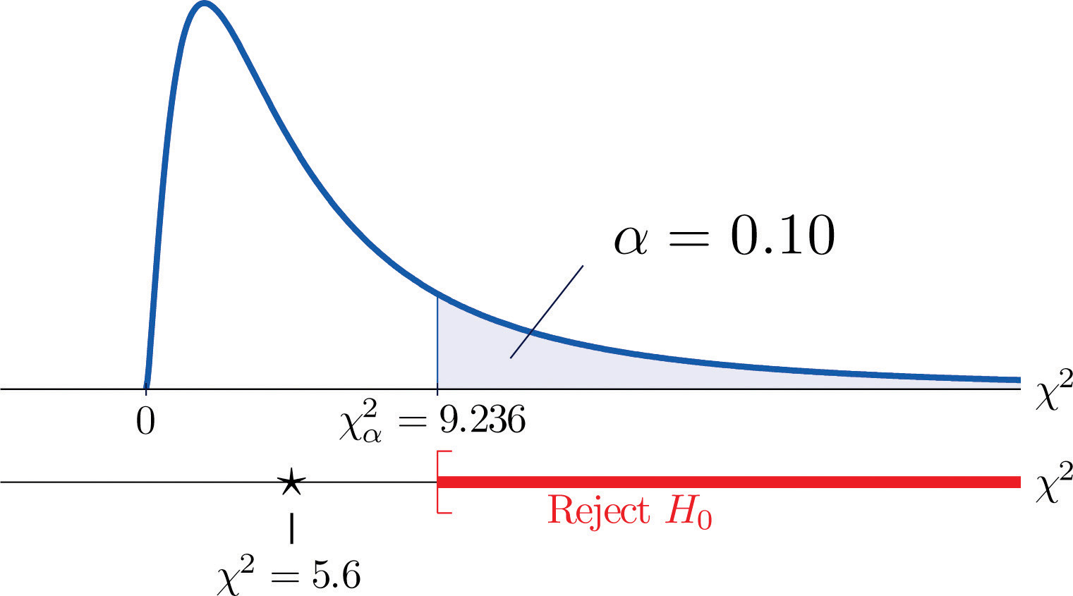
We would reject the null hypothesis that the die is fair only if the number is large, so the test is right-tailed. In this example the random variable has the chi-square distribution with five degrees of freedom. If we had decided at the outset to test at the 10% level of significance, the critical value defining the rejection region would be, reading from Figure 12.4 "Critical Values of Chi-Square Distributions", , so that the rejection region would be the interval When we compute the value of the standardized test statistic using the numbers in the last two columns of Table 11.9 "Updated Die Contingency Table", we obtain
Since 5.6 < 9.236 the decision is not to reject H0. See Figure 11.5 "Balanced Die". The data do not provide sufficient evidence, at the 10% level of significance, to conclude that the die is loaded.
Figure 11.5 Balanced Die
In the general situation we consider a discrete random variable that can take I different values, , for which the default assumption is that the probability distribution is
We wish to test the hypotheses
We take a sample of size n and obtain a list of observed frequencies. This is shown in Table 11.10 "General Contingency Table". Based on the assumed probability distribution we also have a list of assumed frequencies, each of which is defined and computed by the formula
Table 11.10 General Contingency Table
| Factor Levels | Assumed Distribution | Observed Frequency |
|---|---|---|
| 1 | p1 | O1 |
| 2 | p2 | O2 |
| ⋮ | ⋮ | ⋮ |
| I | pI | OI |
Table 11.10 "General Contingency Table" is updated to Table 11.11 "Updated General Contingency Table" by adding the expected frequency for each value of X. To simplify the notation we drop indices for the observed and expected frequencies and represent Table 11.11 "Updated General Contingency Table" by Table 11.12 "Simplified Updated General Contingency Table".
Table 11.11 Updated General Contingency Table
| Factor Levels | Assumed Distribution | Observed Freq. | Expected Freq. |
|---|---|---|---|
| 1 | p1 | O1 | E1 |
| 2 | p2 | O2 | E2 |
| ⋮ | ⋮ | ⋮ | ⋮ |
| I | pI | OI | EI |
Table 11.12 Simplified Updated General Contingency Table
| Factor Levels | Assumed Distribution | Observed Freq. | Expected Freq. |
|---|---|---|---|
| 1 | p1 | O | E |
| 2 | p2 | O | E |
| ⋮ | ⋮ | ⋮ | ⋮ |
| I | pI | O | E |
Here is the test statistic for the general hypothesis based on Table 11.12 "Simplified Updated General Contingency Table", together with the conditions that it follow a chi-square distribution.
Test Statistic for Testing Goodness of Fit to a Discrete Probability Distribution
where the sum is over all the rows of the table (one for each value of X).
If
- the true probability distribution of X is as assumed, and
- the observed count O of each cell in Table 11.12 "Simplified Updated General Contingency Table" is at least 5,
then approximately follows a chi-square distribution with degrees of freedom.
The test is known as a goodness-of-fit test since it tests the null hypothesis that the sample fits the assumed probability distribution well. It is always right-tailed, since deviation from the assumed probability distribution corresponds to large values of
Testing is done using either of the usual five-step procedures.
Example 2
Table 11.13 "Ethnic Groups in the Census Year" shows the distribution of various ethnic groups in the population of a particular state based on a decennial U.S. census. Five years later a random sample of 2,500 residents of the state was taken, with the results given in Table 11.14 "Sample Data Five Years After the Census Year" (along with the probability distribution from the census year). Test, at the 1% level of significance, whether there is sufficient evidence in the sample to conclude that the distribution of ethnic groups in this state five years after the census had changed from that in the census year.
Table 11.13 Ethnic Groups in the Census Year
| Ethnicity | White | Black | Amer.-Indian | Hispanic | Asian | Others |
|---|---|---|---|---|---|---|
| Proportion | 0.743 | 0.216 | 0.012 | 0.012 | 0.008 | 0.009 |
Table 11.14 Sample Data Five Years After the Census Year
| Ethnicity | Assumed Distribution | Observed Frequency |
|---|---|---|
| White | 0.743 | 1732 |
| Black | 0.216 | 538 |
| American-Indian | 0.012 | 32 |
| Hispanic | 0.012 | 42 |
| Asian | 0.008 | 133 |
| Others | 0.009 | 23 |
Solution:
We test using the critical value approach.
-
Step 1. The hypotheses of interest in this case can be expressed as
- Step 2. The distribution is chi-square.
-
Step 3. To compute the value of the test statistic we must first compute the expected number for each row of Table 11.14 "Sample Data Five Years After the Census Year". Since n = 2500, using the formula and the values of pi from either Table 11.13 "Ethnic Groups in the Census Year" or Table 11.14 "Sample Data Five Years After the Census Year",
Table 11.14 "Sample Data Five Years After the Census Year" is updated to Table 11.15 "Observed and Expected Frequencies Five Years After the Census Year".
Table 11.15 Observed and Expected Frequencies Five Years After the Census Year
Ethnicity Assumed Dist. Observed Freq. Expected Freq. White 0.743 1732 1857.5 Black 0.216 538 540 American-Indian 0.012 32 30 Hispanic 0.012 42 30 Asian 0.008 133 20 Others 0.009 23 22.5 The value of the test statistic is
-
Since the random variable takes six values, I = 6. Thus the test statistic follows the chi-square distribution with degrees of freedom.
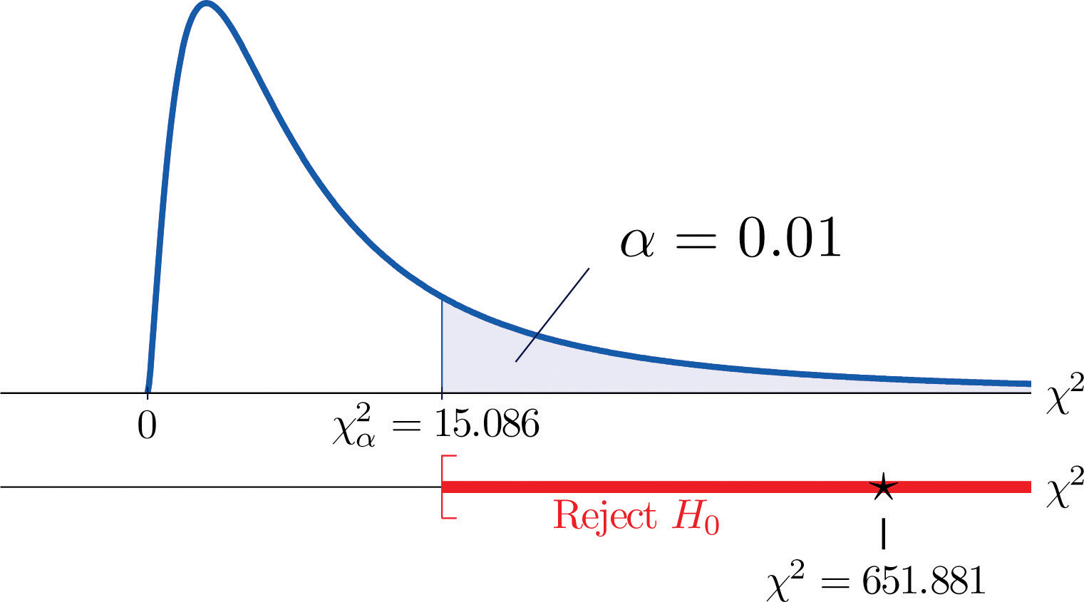
Since the test is right-tailed, the critical value is Reading from Figure 12.4 "Critical Values of Chi-Square Distributions", , so the rejection region is
- Since 651.881 > 15.086 the decision is to reject the null hypothesis. See Figure 11.6. The data provide sufficient evidence, at the 1% level of significance, to conclude that the ethnic distribution in this state has changed in the five years since the U.S. census.
Figure 11.6 Note 11.15 "Example 2"
Key Takeaway
- The chi-square goodness-of-fit testA test based on a chi-square statistic to check whether a sample is taken from a population with a hypothesized probability distribution. can be used to evaluate the hypothesis that a sample is taken from a population with an assumed specific probability distribution.
Exercises
-
A data sample is sorted into five categories with an assumed probability distribution.
Factor Levels Assumed Distribution Observed Frequency 1 10 2 35 3 45 4 10 - Find the size n of the sample.
- Find the expected number E of observations for each level, if the sampled population has a probability distribution as assumed (that is, just use the formula ).
- Find the chi-square test statistic
- Find the number of degrees of freedom of the chi-square test statistic.
-
A data sample is sorted into five categories with an assumed probability distribution.
Factor Levels Assumed Distribution Observed Frequency 1 23 2 30 3 19 4 8 5 10 - Find the size n of the sample.
- Find the expected number E of observations for each level, if the sampled population has a probability distribution as assumed (that is, just use the formula ).
- Find the chi-square test statistic
- Find the number of degrees of freedom of the chi-square test statistic.
Basic
-
Retailers of collectible postage stamps often buy their stamps in large quantities by weight at auctions. The prices the retailers are willing to pay depend on how old the postage stamps are. Many collectible postage stamps at auctions are described by the proportions of stamps issued at various periods in the past. Generally the older the stamps the higher the value. At one particular auction, a lot of collectible stamps is advertised to have the age distribution given in the table provided. A retail buyer took a sample of 73 stamps from the lot and sorted them by age. The results are given in the table provided. Test, at the 5% level of significance, whether there is sufficient evidence in the data to conclude that the age distribution of the lot is different from what was claimed by the seller.
Year Claimed Distribution Observed Frequency Before 1940 0.10 6 1940 to 1959 0.25 15 1960 to 1979 0.45 30 After 1979 0.20 22 -
The litter size of Bengal tigers is typically two or three cubs, but it can vary between one and four. Based on long-term observations, the litter size of Bengal tigers in the wild has the distribution given in the table provided. A zoologist believes that Bengal tigers in captivity tend to have different (possibly smaller) litter sizes from those in the wild. To verify this belief, the zoologist searched all data sources and found 316 litter size records of Bengal tigers in captivity. The results are given in the table provided. Test, at the 5% level of significance, whether there is sufficient evidence in the data to conclude that the distribution of litter sizes in captivity differs from that in the wild.
Litter Size Wild Litter Distribution Observed Frequency 1 0.11 41 2 0.69 243 3 0.18 27 4 0.02 5 -
An online shoe retailer sells men’s shoes in sizes 8 to 13. In the past orders for the different shoe sizes have followed the distribution given in the table provided. The management believes that recent marketing efforts may have expanded their customer base and, as a result, there may be a shift in the size distribution for future orders. To have a better understanding of its future sales, the shoe seller examined 1,040 sales records of recent orders and noted the sizes of the shoes ordered. The results are given in the table provided. Test, at the 1% level of significance, whether there is sufficient evidence in the data to conclude that the shoe size distribution of future sales will differ from the historic one.
Shoe Size Past Size Distribution Recent Size Frequency 8.0 0.03 25 8.5 0.06 43 9.0 0.09 88 9.5 0.19 221 10.0 0.23 272 10.5 0.14 150 11.0 0.10 107 11.5 0.06 51 12.0 0.05 37 12.5 0.03 35 13.0 0.02 11 -
An online shoe retailer sells women’s shoes in sizes 5 to 10. In the past orders for the different shoe sizes have followed the distribution given in the table provided. The management believes that recent marketing efforts may have expanded their customer base and, as a result, there may be a shift in the size distribution for future orders. To have a better understanding of its future sales, the shoe seller examined 1,174 sales records of recent orders and noted the sizes of the shoes ordered. The results are given in the table provided. Test, at the 1% level of significance, whether there is sufficient evidence in the data to conclude that the shoe size distribution of future sales will differ from the historic one.
Shoe Size Past Size Distribution Recent Size Frequency 5.0 0.02 20 5.5 0.03 23 6.0 0.07 88 6.5 0.08 90 7.0 0.20 222 7.5 0.20 258 8.0 0.15 177 8.5 0.11 121 9.0 0.08 91 9.5 0.04 53 10.0 0.02 31 -
A chess opening is a sequence of moves at the beginning of a chess game. There are many well-studied named openings in chess literature. French Defense is one of the most popular openings for black, although it is considered a relatively weak opening since it gives black probability 0.344 of winning, probability 0.405 of losing, and probability 0.251 of drawing. A chess master believes that he has discovered a new variation of French Defense that may alter the probability distribution of the outcome of the game. In his many Internet chess games in the last two years, he was able to apply the new variation in 77 games. The wins, losses, and draws in the 77 games are given in the table provided. Test, at the 5% level of significance, whether there is sufficient evidence in the data to conclude that the newly discovered variation of French Defense alters the probability distribution of the result of the game.
Result for Black Probability Distribution New Variation Wins Win 0.344 31 Loss 0.405 25 Draw 0.251 21 -
The Department of Parks and Wildlife stocks a large lake with fish every six years. It is determined that a healthy diversity of fish in the lake should consist of 10% largemouth bass, 15% smallmouth bass, 10% striped bass, 10% trout, and 20% catfish. Therefore each time the lake is stocked, the fish population in the lake is restored to maintain that particular distribution. Every three years, the department conducts a study to see whether the distribution of the fish in the lake has shifted away from the target proportions. In one particular year, a research group from the department observed a sample of 292 fish from the lake with the results given in the table provided. Test, at the 5% level of significance, whether there is sufficient evidence in the data to conclude that the fish population distribution has shifted since the last stocking.
Fish Target Distribution Fish in Sample Largemouth Bass 0.10 14 Smallmouth Bass 0.15 49 Striped Bass 0.10 21 Trout 0.10 22 Catfish 0.20 75 Other 0.35 111
Applications
-
Large Data Set 4 records the result of 500 tosses of six-sided die. Test, at the 10% level of significance, whether there is sufficient evidence in the data to conclude that the die is not “fair” (or “balanced”), that is, that the probability distribution differs from probability 1/6 for each of the six faces on the die.
Large Data Set Exercise
Answers
-
- n = 100,
- E = 10, E = 40, E = 40, E = 10;
- ,
-
-
, , do not reject H0
-
-
, , reject H0
-
-
, , do not reject H0
-
-
Rejection Region: Decision: Fail to reject H0 of balance.