This is “The Linear Correlation Coefficient”, section 10.2 from the book Beginning Statistics (v. 1.0). For details on it (including licensing), click here.
For more information on the source of this book, or why it is available for free, please see the project's home page. You can browse or download additional books there. To download a .zip file containing this book to use offline, simply click here.


10.2 The Linear Correlation Coefficient
Learning Objective
- To learn what the linear correlation coefficient is, how to compute it, and what it tells us about the relationship between two variables x and y.
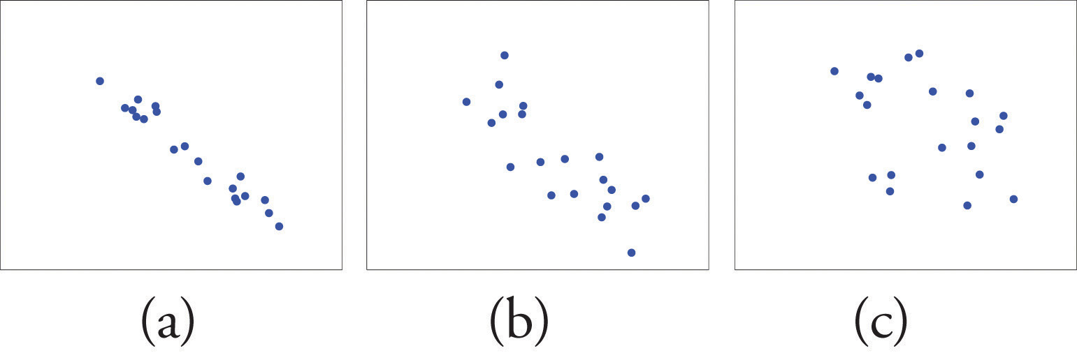
Figure 10.3 "Linear Relationships of Varying Strengths" illustrates linear relationships between two variables x and y of varying strengths. It is visually apparent that in the situation in panel (a), x could serve as a useful predictor of y, it would be less useful in the situation illustrated in panel (b), and in the situation of panel (c) the linear relationship is so weak as to be practically nonexistent. The linear correlation coefficient is a number computed directly from the data that measures the strength of the linear relationship between the two variables x and y.
Figure 10.3 Linear Relationships of Varying Strengths
Definition
The linear correlation coefficientA number computed directly from the data that measures the strength of the linear relationship between the two variables x and y. for a collection of n pairs of numbers in a sample is the number r given by the formula
where
The linear correlation coefficient has the following properties, illustrated in Figure 10.4 "Linear Correlation Coefficient ":
- The value of r lies between −1 and 1, inclusive.
- The sign of r indicates the direction of the linear relationship between x and y:
- If then y tends to decrease as x is increased.
- If then y tends to increase as x is increased.
- The size of |r| indicates the strength of the linear relationship between x and y:
- If |r| is near 1 (that is, if r is near either 1 or −1) then the linear relationship between x and y is strong.
- If |r| is near 0 (that is, if r is near 0 and of either sign) then the linear relationship between x and y is weak.
Figure 10.4 Linear Correlation Coefficient R
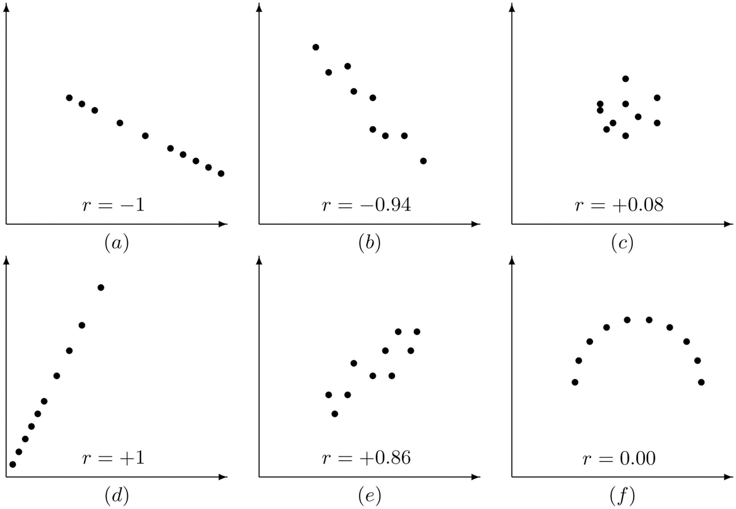
Pay particular attention to panel (f) in Figure 10.4 "Linear Correlation Coefficient ". It shows a perfectly deterministic relationship between x and y, but because the relationship is not linear. (In this particular case the points lie on the top half of a circle.)
Example 1
Compute the linear correlation coefficient for the height and weight pairs plotted in Figure 10.2 "Plot of Height and Weight Pairs".
Solution:
Even for small data sets like this one computations are too long to do completely by hand. In actual practice the data are entered into a calculator or computer and a statistics program is used. In order to clarify the meaning of the formulas we will display the data and related quantities in tabular form. For each pair we compute three numbers: x2, , and y2, as shown in the table provided. In the last line of the table we have the sum of the numbers in each column. Using them we compute:
| x | y | x2 | y2 | ||
|---|---|---|---|---|---|
| 68 | 151 | 4624 | 10268 | 22801 | |
| 69 | 146 | 4761 | 10074 | 21316 | |
| 70 | 157 | 4900 | 10990 | 24649 | |
| 70 | 164 | 4900 | 11480 | 26896 | |
| 71 | 171 | 5041 | 12141 | 29241 | |
| 72 | 160 | 5184 | 11520 | 25600 | |
| 72 | 163 | 5184 | 11736 | 26569 | |
| 72 | 180 | 5184 | 12960 | 32400 | |
| 73 | 170 | 5329 | 12410 | 28900 | |
| 73 | 175 | 5329 | 12775 | 30625 | |
| 74 | 178 | 5476 | 13172 | 31684 | |
| 75 | 188 | 5625 | 14100 | 35344 | |
| Σ | 859 | 2003 | 61537 | 143626 | 336025 |
so that
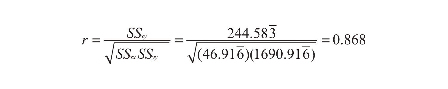
The number quantifies what is visually apparent from Figure 10.2 "Plot of Height and Weight Pairs": weights tends to increase linearly with height (r is positive) and although the relationship is not perfect, it is reasonably strong (r is near 1).
Key Takeaways
- The linear correlation coefficient measures the strength and direction of the linear relationship between two variables x and y.
- The sign of the linear correlation coefficient indicates the direction of the linear relationship between x and y.
- When r is near 1 or −1 the linear relationship is strong; when it is near 0 the linear relationship is weak.
Exercises
-
For the sample data
- Draw the scatter plot.
- Based on the scatter plot, predict the sign of the linear correlation coefficient. Explain your answer.
- Compute the linear correlation coefficient and compare its sign to your answer to part (b).
-
For the sample data
- Draw the scatter plot.
- Based on the scatter plot, predict the sign of the linear correlation coefficient. Explain your answer.
- Compute the linear correlation coefficient and compare its sign to your answer to part (b).
-
For the sample data
- Draw the scatter plot.
- Based on the scatter plot, predict the sign of the linear correlation coefficient. Explain your answer.
- Compute the linear correlation coefficient and compare its sign to your answer to part (b).
-
For the sample data
- Draw the scatter plot.
- Based on the scatter plot, predict the sign of the linear correlation coefficient. Explain your answer.
- Compute the linear correlation coefficient and compare its sign to your answer to part (b).
-
For the sample data
- Draw the scatter plot.
- Based on the scatter plot, predict the sign of the linear correlation coefficient. Explain your answer.
- Compute the linear correlation coefficient and compare its sign to your answer to part (b).
-
For the sample data
- Draw the scatter plot.
- Based on the scatter plot, predict the sign of the linear correlation coefficient. Explain your answer.
- Compute the linear correlation coefficient and compare its sign to your answer to part (b).
-
Compute the linear correlation coefficient for the sample data summarized by the following information:
-
Compute the linear correlation coefficient for the sample data summarized by the following information:
-
Compute the linear correlation coefficient for the sample data summarized by the following information:
-
Compute the linear correlation coefficient for the sample data summarized by the following information:
Basic
With the exception of the exercises at the end of Section 10.3 "Modelling Linear Relationships with Randomness Present", the first Basic exercise in each of the following sections through Section 10.7 "Estimation and Prediction" uses the data from the first exercise here, the second Basic exercise uses the data from the second exercise here, and so on, and similarly for the Application exercises. Save your computations done on these exercises so that you do not need to repeat them later.
-
The age x in months and vocabulary y were measured for six children, with the results shown in the table.
Compute the linear correlation coefficient for these sample data and interpret its meaning in the context of the problem.
-
The curb weight x in hundreds of pounds and braking distance y in feet, at 50 miles per hour on dry pavement, were measured for five vehicles, with the results shown in the table.
Compute the linear correlation coefficient for these sample data and interpret its meaning in the context of the problem.
-
The age x and resting heart rate y were measured for ten men, with the results shown in the table.
Compute the linear correlation coefficient for these sample data and interpret its meaning in the context of the problem.
-
The wind speed x in miles per hour and wave height y in feet were measured under various conditions on an enclosed deep water sea, with the results shown in the table,
Compute the linear correlation coefficient for these sample data and interpret its meaning in the context of the problem.
-
The advertising expenditure x and sales y in thousands of dollars for a small retail business in its first eight years in operation are shown in the table.
Compute the linear correlation coefficient for these sample data and interpret its meaning in the context of the problem.
-
The height x at age 2 and y at age 20, both in inches, for ten women are tabulated in the table.
Compute the linear correlation coefficient for these sample data and interpret its meaning in the context of the problem.
-
The course average x just before a final exam and the score y on the final exam were recorded for 15 randomly selected students in a large physics class, with the results shown in the table.
Compute the linear correlation coefficient for these sample data and interpret its meaning in the context of the problem.
-
The table shows the acres x of corn planted and acres y of corn harvested, in millions of acres, in a particular country in ten successive years.
Compute the linear correlation coefficient for these sample data and interpret its meaning in the context of the problem.
-
Fifty male subjects drank a measured amount x (in ounces) of a medication and the concentration y (in percent) in their blood of the active ingredient was measured 30 minutes later. The sample data are summarized by the following information.
Compute the linear correlation coefficient for these sample data and interpret its meaning in the context of the problem.
-
In an effort to produce a formula for estimating the age of large free-standing oak trees non-invasively, the girth x (in inches) five feet off the ground of 15 such trees of known age y (in years) was measured. The sample data are summarized by the following information.
Compute the linear correlation coefficient for these sample data and interpret its meaning in the context of the problem.
-
Construction standards specify the strength of concrete 28 days after it is poured. For 30 samples of various types of concrete the strength x after 3 days and the strength y after 28 days (both in hundreds of pounds per square inch) were measured. The sample data are summarized by the following information.
Compute the linear correlation coefficient for these sample data and interpret its meaning in the context of the problem.
-
Power-generating facilities used forecasts of temperature to forecast energy demand. The average temperature x (degrees Fahrenheit) and the day’s energy demand y (million watt-hours) were recorded on 40 randomly selected winter days in the region served by a power company. The sample data are summarized by the following information.
Compute the linear correlation coefficient for these sample data and interpret its meaning in the context of the problem.
Applications
-
In each case state whether you expect the two variables x and y indicated to have positive, negative, or zero correlation.
- the number x of pages in a book and the age y of the author
- the number x of pages in a book and the age y of the intended reader
- the weight x of an automobile and the fuel economy y in miles per gallon
- the weight x of an automobile and the reading y on its odometer
- the amount x of a sedative a person took an hour ago and the time y it takes him to respond to a stimulus
-
In each case state whether you expect the two variables x and y indicated to have positive, negative, or zero correlation.
- the length x of time an emergency flare will burn and the length y of time the match used to light it burned
- the average length x of time that calls to a retail call center are on hold one day and the number y of calls received that day
- the length x of a regularly scheduled commercial flight between two cities and the headwind y encountered by the aircraft
- the value x of a house and the its size y in square feet
- the average temperature x on a winter day and the energy consumption y of the furnace
-
Changing the units of measurement on two variables x and y should not change the linear correlation coefficient. Moreover, most change of units amount to simply multiplying one unit by the other (for example, 1 foot = 12 inches). Multiply each x value in the table in Exercise 1 by two and compute the linear correlation coefficient for the new data set. Compare the new value of r to the one for the original data.
-
Refer to the previous exercise. Multiply each x value in the table in Exercise 2 by two, multiply each y value by three, and compute the linear correlation coefficient for the new data set. Compare the new value of r to the one for the original data.
-
Reversing the roles of x and y in the data set of Exercise 1 produces the data set
Compute the linear correlation coefficient of the new set of data and compare it to what you got in Exercise 1.
-
In the context of the previous problem, look at the formula for r and see if you can tell why what you observed there must be true for every data set.
Additional Exercises
-
Large Data Set 1 lists the SAT scores and GPAs of 1,000 students. Compute the linear correlation coefficient r. Compare its value to your comments on the appearance and strength of any linear trend in the scatter diagram that you constructed in the first large data set problem for Section 10.1 "Linear Relationships Between Variables".
-
Large Data Set 12 lists the golf scores on one round of golf for 75 golfers first using their own original clubs, then using clubs of a new, experimental design (after two months of familiarization with the new clubs). Compute the linear correlation coefficient r. Compare its value to your comments on the appearance and strength of any linear trend in the scatter diagram that you constructed in the second large data set problem for Section 10.1 "Linear Relationships Between Variables".
http://www.flatworldknowledge.com/sites/all/files/data12.xls
-
Large Data Set 13 records the number of bidders and sales price of a particular type of antique grandfather clock at 60 auctions. Compute the linear correlation coefficient r. Compare its value to your comments on the appearance and strength of any linear trend in the scatter diagram that you constructed in the third large data set problem for Section 10.1 "Linear Relationships Between Variables".
http://www.flatworldknowledge.com/sites/all/files/data13.xls
Large Data Set Exercises
Answers
-
-
-
-
-
-
-
0.875
-
-
−0.846
-
-
0.948
-
-
0.709
-
-
0.832
-
-
0.751
-
-
0.965
-
-
0.992
-
-
- zero
- positive
- negative
- zero
- positive
-
-
same value
-
-
same value
-