This is “Small Sample Tests for a Population Mean”, section 8.4 from the book Beginning Statistics (v. 1.0). For details on it (including licensing), click here.
For more information on the source of this book, or why it is available for free, please see the project's home page. You can browse or download additional books there. To download a .zip file containing this book to use offline, simply click here.


8.4 Small Sample Tests for a Population Mean
Learning Objective
- To learn how to apply the five-step test procedure for test of hypotheses concerning a population mean when the sample size is small.
In the previous section hypotheses testing for population means was described in the case of large samples. The statistical validity of the tests was insured by the Central Limit Theorem, with essentially no assumptions on the distribution of the population. When sample sizes are small, as is often the case in practice, the Central Limit Theorem does not apply. One must then impose stricter assumptions on the population to give statistical validity to the test procedure. One common assumption is that the population from which the sample is taken has a normal probability distribution to begin with. Under such circumstances, if the population standard deviation is known, then the test statistic still has the standard normal distribution, as in the previous two sections. If σ is unknown and is approximated by the sample standard deviation s, then the resulting test statistic follows Student’s t-distribution with degrees of freedom.
Standardized Test Statistics for Small Sample Hypothesis Tests Concerning a Single Population Mean
The first test statistic (σ known) has the standard normal distribution.
The second test statistic (σ unknown) has Student’s t-distribution with degrees of freedom.
The population must be normally distributed.
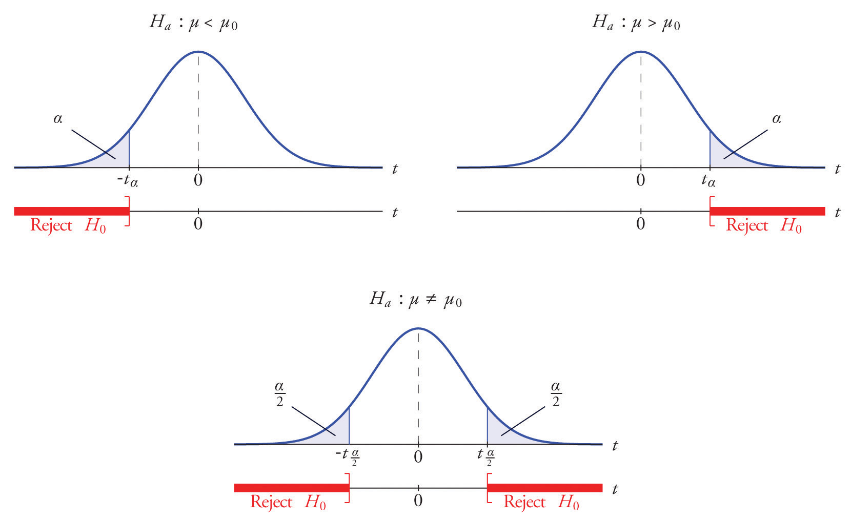
The distribution of the second standardized test statistic (the one containing s) and the corresponding rejection region for each form of the alternative hypothesis (left-tailed, right-tailed, or two-tailed), is shown in Figure 8.11 "Distribution of the Standardized Test Statistic and the Rejection Region". This is just like Figure 8.4 "Distribution of the Standardized Test Statistic and the Rejection Region", except that now the critical values are from the t-distribution. Figure 8.4 "Distribution of the Standardized Test Statistic and the Rejection Region" still applies to the first standardized test statistic (the one containing σ) since it follows the standard normal distribution.
Figure 8.11 Distribution of the Standardized Test Statistic and the Rejection Region
The p-value of a test of hypotheses for which the test statistic has Student’s t-distribution can be computed using statistical software, but it is impractical to do so using tables, since that would require 30 tables analogous to Figure 12.2 "Cumulative Normal Probability", one for each degree of freedom from 1 to 30. Figure 12.3 "Critical Values of " can be used to approximate the p-value of such a test, and this is typically adequate for making a decision using the p-value approach to hypothesis testing, although not always. For this reason the tests in the two examples in this section will be made following the critical value approach to hypothesis testing summarized at the end of Section 8.1 "The Elements of Hypothesis Testing", but after each one we will show how the p-value approach could have been used.
Example 10
The price of a popular tennis racket at a national chain store is $179. Portia bought five of the same racket at an online auction site for the following prices:
Assuming that the auction prices of rackets are normally distributed, determine whether there is sufficient evidence in the sample, at the 5% level of significance, to conclude that the average price of the racket is less than $179 if purchased at an online auction.
Solution:
-
Step 1. The assertion for which evidence must be provided is that the average online price μ is less than the average price in retail stores, so the hypothesis test is
-
Step 2. The sample is small and the population standard deviation is unknown. Thus the test statistic is
and has the Student t-distribution with degrees of freedom.
-
Step 3. From the data we compute and s = 10.39. Inserting these values into the formula for the test statistic gives
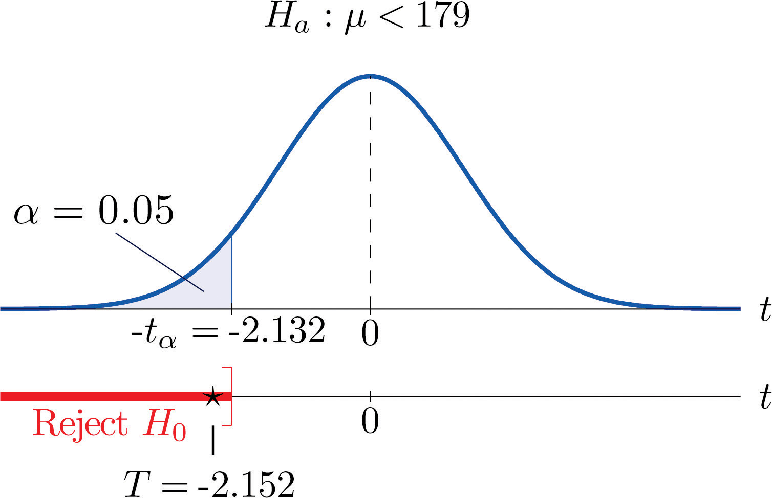
- Step 4. Since the symbol in Ha is “<” this is a left-tailed test, so there is a single critical value, Reading from the row labeled in Figure 12.3 "Critical Values of " its value is −2.132. The rejection region is
-
Step 5. As shown in Figure 8.12 "Rejection Region and Test Statistic for " the test statistic falls in the rejection region. The decision is to reject H0. In the context of the problem our conclusion is:
The data provide sufficient evidence, at the 5% level of significance, to conclude that the average price of such rackets purchased at online auctions is less than $179.
Figure 8.12 Rejection Region and Test Statistic for Note 8.42 "Example 10"
To perform the test in Note 8.42 "Example 10" using the p-value approach, look in the row in Figure 12.3 "Critical Values of " with the heading and search for the two t-values that bracket the unsigned value 2.152 of the test statistic. They are 2.132 and 2.776, in the columns with headings t0.050 and t0.025. They cut off right tails of area 0.050 and 0.025, so because 2.152 is between them it must cut off a tail of area between 0.050 and 0.025. By symmetry −2.152 cuts off a left tail of area between 0.050 and 0.025, hence the p-value corresponding to is between 0.025 and 0.05. Although its precise value is unknown, it must be less than , so the decision is to reject H0.
Example 11
A small component in an electronic device has two small holes where another tiny part is fitted. In the manufacturing process the average distance between the two holes must be tightly controlled at 0.02 mm, else many units would be defective and wasted. Many times throughout the day quality control engineers take a small sample of the components from the production line, measure the distance between the two holes, and make adjustments if needed. Suppose at one time four units are taken and the distances are measured as
Determine, at the 1% level of significance, if there is sufficient evidence in the sample to conclude that an adjustment is needed. Assume the distances of interest are normally distributed.
Solution:
-
Step 1. The assumption is that the process is under control unless there is strong evidence to the contrary. Since a deviation of the average distance to either side is undesirable, the relevant test is
where μ denotes the mean distance between the holes.
-
Step 2. The sample is small and the population standard deviation is unknown. Thus the test statistic is
and has the Student t-distribution with degrees of freedom.
-
Step 3. From the data we compute and s = 0.00171. Inserting these values into the formula for the test statistic gives
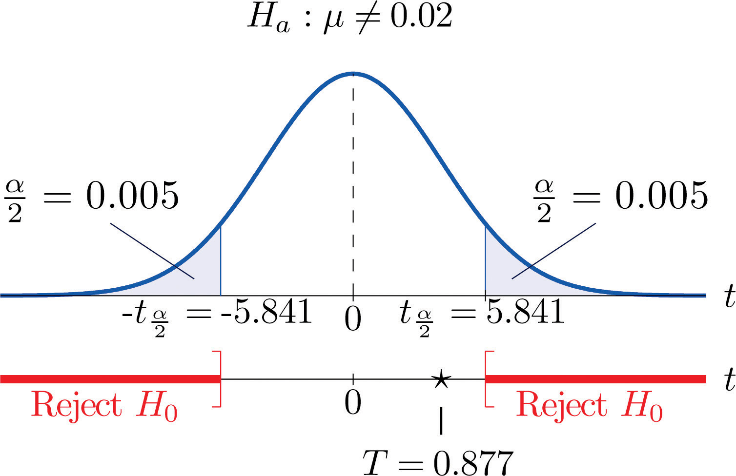
- Step 4. Since the symbol in Ha is “≠” this is a two-tailed test, so there are two critical values, Reading from the row in Figure 12.3 "Critical Values of " labeled their values are The rejection region is
-
Step 5. As shown in Figure 8.13 "Rejection Region and Test Statistic for " the test statistic does not fall in the rejection region. The decision is not to reject H0. In the context of the problem our conclusion is:
The data do not provide sufficient evidence, at the 1% level of significance, to conclude that the mean distance between the holes in the component differs from 0.02 mm.
Figure 8.13 Rejection Region and Test Statistic for Note 8.43 "Example 11"
To perform the test in Note 8.43 "Example 11" using the p-value approach, look in the row in Figure 12.3 "Critical Values of " with the heading and search for the two t-values that bracket the value 0.877 of the test statistic. Actually 0.877 is smaller than the smallest number in the row, which is 0.978, in the column with heading t0.200. The value 0.978 cuts off a right tail of area 0.200, so because 0.877 is to its left it must cut off a tail of area greater than 0.200. Thus the p-value, which is the double of the area cut off (since the test is two-tailed), is greater than 0.400. Although its precise value is unknown, it must be greater than , so the decision is not to reject H0.
Key Takeaways
- There are two formulas for the test statistic in testing hypotheses about a population mean with small samples. One test statistic follows the standard normal distribution, the other Student’s t-distribution.
- The population standard deviation is used if it is known, otherwise the sample standard deviation is used.
- Either five-step procedure, critical value or p-value approach, is used with either test statistic.
Exercises
-
Find the rejection region (for the standardized test statistic) for each hypothesis test based on the information given. The population is normally distributed.
- vs. @ , n = 12, σ = 2.2.
- vs. @ , n = 6, σ unknown.
- vs. @ , n = 24, σ unknown.
- vs. @ , n = 8, σ = 1.7.
-
Find the rejection region (for the standardized test statistic) for each hypothesis test based on the information given. The population is normally distributed.
- vs. @ , n = 26, σ = 0.94.
- vs. @ , n = 4, σ unknown.
- vs. @ , n = 18, σ = 1.1.
- vs. @ , n = 23, σ unknown.
-
Find the rejection region (for the standardized test statistic) for each hypothesis test based on the information given. The population is normally distributed. Identify the test as left-tailed, right-tailed, or two-tailed.
- vs. @ , n = 29, σ unknown.
- vs. @ , n = 15, σ = 1.9.
- vs. @ , n = 12, σ unknown.
- vs. @ , n = 27, σ unknown.
-
Find the rejection region (for the standardized test statistic) for each hypothesis test based on the information given. The population is normally distributed. Identify the test as left-tailed, right-tailed, or two-tailed.
- vs. @ , n = 8, σ unknown.
- vs. @ n = 22, σ unknown.
- vs. @ , n = 21, σ unknown.
- vs. @ , n = 14, σ = 0.026.
-
A random sample of size 20 drawn from a normal population yielded the following results: , s = 1.33.
- Test vs. @
- Estimate the observed significance of the test in part (a) and state a decision based on the p-value approach to hypothesis testing.
-
A random sample of size 16 drawn from a normal population yielded the following results: , s = 1.07.
- Test vs. @
- Estimate the observed significance of the test in part (a) and state a decision based on the p-value approach to hypothesis testing.
-
A random sample of size 8 drawn from a normal population yielded the following results: , s = 46.
- Test vs. @
- Estimate the observed significance of the test in part (a) and state a decision based on the p-value approach to hypothesis testing.
-
A random sample of size 12 drawn from a normal population yielded the following results: , s = 0.63.
- Test vs. @
- Estimate the observed significance of the test in part (a) and state a decision based on the p-value approach to hypothesis testing.
Basic
-
Researchers wish to test the efficacy of a program intended to reduce the length of labor in childbirth. The accepted mean labor time in the birth of a first child is 15.3 hours. The mean length of the labors of 13 first-time mothers in a pilot program was 8.8 hours with standard deviation 3.1 hours. Assuming a normal distribution of times of labor, test at the 10% level of significance test whether the mean labor time for all women following this program is less than 15.3 hours.
-
A dairy farm uses the somatic cell count (SCC) report on the milk it provides to a processor as one way to monitor the health of its herd. The mean SCC from five samples of raw milk was 250,000 cells per milliliter with standard deviation 37,500 cell/ml. Test whether these data provide sufficient evidence, at the 10% level of significance, to conclude that the mean SCC of all milk produced at the dairy exceeds that in the previous report, 210,250 cell/ml. Assume a normal distribution of SCC.
-
Six coins of the same type are discovered at an archaeological site. If their weights on average are significantly different from 5.25 grams then it can be assumed that their provenance is not the site itself. The coins are weighed and have mean 4.73 g with sample standard deviation 0.18 g. Perform the relevant test at the 0.1% (1/10th of 1%) level of significance, assuming a normal distribution of weights of all such coins.
-
An economist wishes to determine whether people are driving less than in the past. In one region of the country the number of miles driven per household per year in the past was 18.59 thousand miles. A sample of 15 households produced a sample mean of 16.23 thousand miles for the last year, with sample standard deviation 4.06 thousand miles. Assuming a normal distribution of household driving distances per year, perform the relevant test at the 5% level of significance.
-
The recommended daily allowance of iron for females aged 19–50 is 18 mg/day. A careful measurement of the daily iron intake of 15 women yielded a mean daily intake of 16.2 mg with sample standard deviation 4.7 mg.
- Assuming that daily iron intake in women is normally distributed, perform the test that the actual mean daily intake for all women is different from 18 mg/day, at the 10% level of significance.
- The sample mean is less than 18, suggesting that the actual population mean is less than 18 mg/day. Perform this test, also at the 10% level of significance. (The computation of the test statistic done in part (a) still applies here.)
-
The target temperature for a hot beverage the moment it is dispensed from a vending machine is 170°F. A sample of ten randomly selected servings from a new machine undergoing a pre-shipment inspection gave mean temperature 173°F with sample standard deviation 6.3°F.
- Assuming that temperature is normally distributed, perform the test that the mean temperature of dispensed beverages is different from 170°F, at the 10% level of significance.
- The sample mean is greater than 170, suggesting that the actual population mean is greater than 170°F. Perform this test, also at the 10% level of significance. (The computation of the test statistic done in part (a) still applies here.)
-
The average number of days to complete recovery from a particular type of knee operation is 123.7 days. From his experience a physician suspects that use of a topical pain medication might be lengthening the recovery time. He randomly selects the records of seven knee surgery patients who used the topical medication. The times to total recovery were:
- Assuming a normal distribution of recovery times, perform the relevant test of hypotheses at the 10% level of significance.
- Would the decision be the same at the 5% level of significance? Answer either by constructing a new rejection region (critical value approach) or by estimating the p-value of the test in part (a) and comparing it to
-
A 24-hour advance prediction of a day’s high temperature is “unbiased” if the long-term average of the error in prediction (true high temperature minus predicted high temperature) is zero. The errors in predictions made by one meteorological station for 20 randomly selected days were:
- Assuming a normal distribution of errors, test the null hypothesis that the predictions are unbiased (the mean of the population of all errors is 0) versus the alternative that it is biased (the population mean is not 0), at the 1% level of significance.
- Would the decision be the same at the 5% level of significance? The 10% level of significance? Answer either by constructing new rejection regions (critical value approach) or by estimating the p-value of the test in part (a) and comparing it to
-
Pasteurized milk may not have a standardized plate count (SPC) above 20,000 colony-forming bacteria per milliliter (cfu/ml). The mean SPC for five samples was 21,500 cfu/ml with sample standard deviation 750 cfu/ml. Test the null hypothesis that the mean SPC for this milk is 20,000 versus the alternative that it is greater than 20,000, at the 10% level of significance. Assume that the SPC follows a normal distribution.
-
One water quality standard for water that is discharged into a particular type of stream or pond is that the average daily water temperature be at most 18°C. Six samples taken throughout the day gave the data:
The sample mean exceeds 18, but perhaps this is only sampling error. Determine whether the data provide sufficient evidence, at the 10% level of significance, to conclude that the mean temperature for the entire day exceeds 18°C.
Applications
-
A calculator has a built-in algorithm for generating a random number according to the standard normal distribution. Twenty-five numbers thus generated have mean 0.15 and sample standard deviation 0.94. Test the null hypothesis that the mean of all numbers so generated is 0 versus the alternative that it is different from 0, at the 20% level of significance. Assume that the numbers do follow a normal distribution.
-
At every setting a high-speed packing machine delivers a product in amounts that vary from container to container with a normal distribution of standard deviation 0.12 ounce. To compare the amount delivered at the current setting to the desired amount 64.1 ounce, a quality inspector randomly selects five containers and measures the contents of each, obtaining sample mean 63.9 ounces and sample standard deviation 0.10 ounce. Test whether the data provide sufficient evidence, at the 5% level of significance, to conclude that the mean of all containers at the current setting is less than 64.1 ounces.
-
A manufacturing company receives a shipment of 1,000 bolts of nominal shear strength 4,350 lb. A quality control inspector selects five bolts at random and measures the shear strength of each. The data are:
- Assuming a normal distribution of shear strengths, test the null hypothesis that the mean shear strength of all bolts in the shipment is 4,350 lb versus the alternative that it is less than 4,350 lb, at the 10% level of significance.
- Estimate the p-value (observed significance) of the test of part (a).
- Compare the p-value found in part (b) to and make a decision based on the p-value approach. Explain fully.
-
A literary historian examines a newly discovered document possibly written by Oberon Theseus. The mean average sentence length of the surviving undisputed works of Oberon Theseus is 48.72 words. The historian counts words in sentences between five successive 101 periods in the document in question to obtain a mean average sentence length of 39.46 words with standard deviation 7.45 words. (Thus the sample size is five.)
- Determine if these data provide sufficient evidence, at the 1% level of significance, to conclude that the mean average sentence length in the document is less than 48.72.
- Estimate the p-value of the test.
- Based on the answers to parts (a) and (b), state whether or not it is likely that the document was written by Oberon Theseus.
Additional Exercises
Answers
-
- or T ≥ 2.571
- T ≥ 1.319
- or Z ≥ 1.645
-
-
- or T ≥ 2.201
- T ≥ 3.435
-
-
- , , , do not reject H0.
- , , do not reject H0.
-
-
- T = 2.398, , , reject H0.
- , , reject H0.
-
-
, , , reject H0.
-
-
, , , reject H0.
-
-
- , , , do not reject H0;
- , , , reject H0;
-
-
- T = 2.069, , , reject H0;
- T = 2.069, , , reject H0.
-
-
T = 4.472, , , reject H0.
-
-
T = 0.798, , , do not reject H0.
-
-
- , , , do not reject H0.
- , do not reject H0
-