This is “Software and Technology Exercise”, section 9.4 from the book Beginning Project Management (v. 1.1). For details on it (including licensing), click here.
For more information on the source of this book, or why it is available for free, please see the project's home page. You can browse or download additional books there. To download a .zip file containing this book to use offline, simply click here.
9.4 Software and Technology Exercise
Learning Objective
- Create a spreadsheet to perform an earned value analysis.
Earned Value Analysis
In this exercise, you apply the formulas of earned value (EV) analysis to the John’s Move project. Complete the exercise by following these instructions:
-
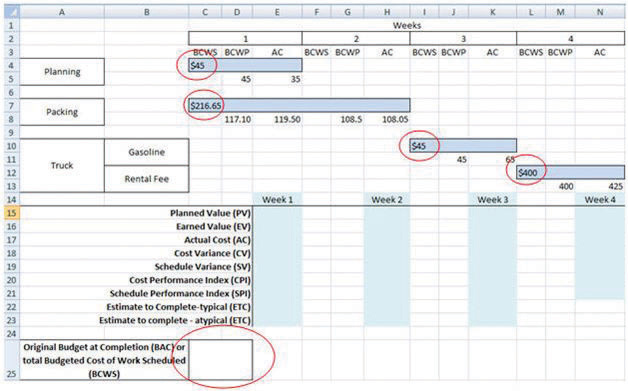
Navigate to the location where the student supplement files are stored and open Ch09EV.xls in a spreadsheet program such as MS Excel. Save the file on your computer as Ch09EVStudentName.xls. Four tasks span four weeks. The budgeted cost of work scheduled (BCWS) is shown at the beginning of each bar, as shown in Figure 9.11 "EV Analysis for John’s Move".
Figure 9.11 EV Analysis for John’s Move
© Microsoft Corporation. All Rights Reserved. Used with permission from Microsoft Corporation.
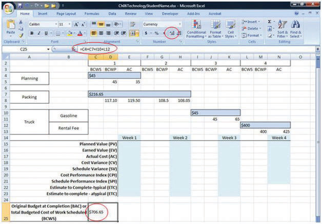
- In cell C25, type =C4+C7+I10+L12 and then press Enter. The sum of the budgeted amounts for each task is the budget at completion (BAC).
-
Click cell C25 to select it. In the Number group, click the Increase Decimal button two times, if necessary, to display two decimal places. See Figure 9.12 "BAC Calculation".
Figure 9.12 BAC Calculation
© Microsoft Corporation. All Rights Reserved. Used with permission from Microsoft Corporation.
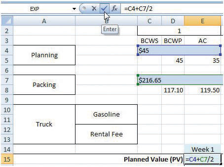
- Click cell E15. Type =C4+C7/2. The planned value (PV) for the first week is the BCWS for the week. In this example, that is all the BCWS for planning and half of the BCWS for packing. The packing task is scheduled to take two weeks. Without further instructions, the budgeted amount is divided equally between the two weeks.
-
Move the mouse pointer to the Enter button on the Formula bar. See Figure 9.13 "PV Calculation for Week 1". Entering formulas by using this button keeps the selection on the current cell.
Figure 9.13 PV Calculation for Week 1
© Microsoft Corporation. All Rights Reserved. Used with permission from Microsoft Corporation.
- On the Formula bar, click the Enter button. The PV is calculated and displayed in cell E15.
- Capture this screen and paste it into a blank word processing document. Save the word processing document as Ch9EVStudentName using the Word 2003 .doc file format.
-
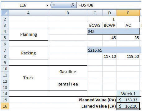
In the spreadsheet, click cell E16. Type =D5+D8 and then, on the Formula bar, click the Enter button. The EV is the sum of the budgeted work that has been performed up to that point in the project. See Figure 9.14 "EV Calculation for Week 1".
Figure 9.14 EV Calculation for Week 1
© Microsoft Corporation. All Rights Reserved. Used with permission from Microsoft Corporation.
- Click cell E17. Type =E5+E8 and then, on the Formula bar, click the Enter button. The actual cost (AC) for week 1 is the sum of the AC for planning and packing that occurred in week 1.
- Click cell E18. Type =E16−E17 and then, on the Formula bar, click the Enter button. The cost variance (CV) for week 1 is the EV minus the AC.
-
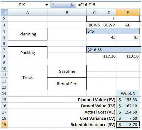
Click cell E19. Type =E16−E15 and then, on the Formula bar, click the Enter button. The schedule variance (SV) for week 1 is EV minus the PV. See Figure 9.15 "AC, CV, and SV Calculations for Week 1".
Figure 9.15 AC, CV, and SV Calculations for Week 1
© Microsoft Corporation. All Rights Reserved. Used with permission from Microsoft Corporation.
-
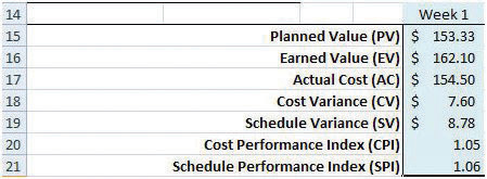
Refer to the definitions of CPI and SPI. Enter formulas in cells E20 and E21 to calculate the CPI and SPI. Recall that formulas begin with an equal sign and use cell names instead of the numbers in those cells. Use the Decrease Decimal or Increase Decimal buttons as needed to display two decimal places. See Figure 9.16 "CPI and SPI Calculations for Week 1".
Figure 9.16 CPI and SPI Calculations for Week 1
© Microsoft Corporation. All Rights Reserved. Used with permission from Microsoft Corporation.
-
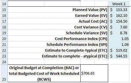
Refer to the definitions of estimate to complete (ETC) for typical and atypical variances in AC. Enter formulas in cells E22 and E23 to calculate the ETC for typical and atypical CV. Recall that the BAC value is in cell C25. Compare your results to Figure 9.17 "ETC at the End of Week 1 for Typical and Atypical AC".
Figure 9.17 ETC at the End of Week 1 for Typical and Atypical AC
© Microsoft Corporation. All Rights Reserved. Used with permission from Microsoft Corporation.
- Click cell H15. Type =E15+C7/2 and then, on the Formula bar, click the Enter button. The PV at the end of week 2 is the sum of PV from the previous week plus the PV for the current week. In this case, the PV for week 2 is the second half of the packing task.
- Click cell H16. Type =E16+G8 and then, on the Formula bar, click the Enter button. The EV at the end of week 2 is the sum of EV from the previous week plus the budgeted cost of work performed (BCWP) for the current week.
- Click cell H17. Type =E17+H8 and then, on the Formula bar, click the Enter button. The AC at the end of week 2 is the sum of AC from the previous week plus the AC for the current week.
-
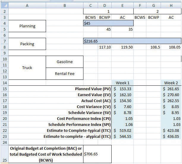
Refer to the definitions for CV, SV, CPI, SPI, and ETC and write formulas in cells H18 through H23 to calculate those values at the end of week 2. See Figure 9.18 "Calculations for Week 2".
Figure 9.18 Calculations for Week 2
© Microsoft Corporation. All Rights Reserved. Used with permission from Microsoft Corporation.
- Capture the screen and paste it into Ch09EVStudentName.doc.
-
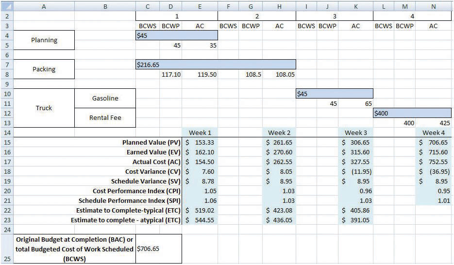
In the spreadsheet, apply what you have learned to perform similar calculations for weeks 3 and 4. See Figure 9.19 "Calculations for Weeks 3 and 4".
Figure 9.19 Calculations for Weeks 3 and 4
© Microsoft Corporation. All Rights Reserved. Used with permission from Microsoft Corporation.
-
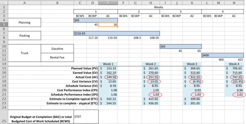
Click cell E5. Type 30 and then, on the Formula bar, click the Enter button. Notice that all the calculations that depend on the AC in this cell are recalculated. See Figure 9.20 "Values That Depend on the AC in Cell E5 Change".
Figure 9.20 Values That Depend on the AC in Cell E5 Change
© Microsoft Corporation. All Rights Reserved. Used with permission from Microsoft Corporation.
- Capture the screen and paste it into Ch09EVStudentName.doc.
Prepare the worksheet for printing:
- In the spreadsheet, on the menu bar, click Page Layout. In the Page Setup group, at the lower right corner, click the Expand button.
-
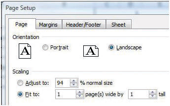
In the Page Setup dialog box, on the Page tab, click the Landscape button and the Fit To button. See Figure 9.21 "Printout Oriented Horizontally and Forced to Fit on One Page".
Figure 9.21 Printout Oriented Horizontally and Forced to Fit on One Page
© Microsoft Corporation. All Rights Reserved. Used with permission from Microsoft Corporation.
-
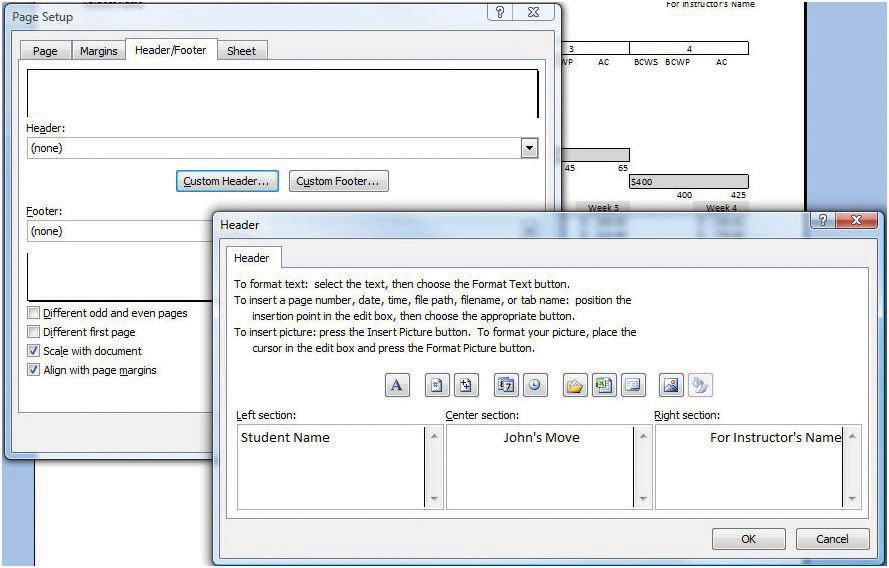
In the Page Setup dialog box, on the Header/Footer tab, click the In the Header dialog box, click the Left section, and then type your name. Click the Center section and then type John’s Move. Click the Right section box and type For InstructorName, substituting your instructor’s name. See Figure 9.22 "Your Name and Your Instructor’s Name in the Header".
Figure 9.22 Your Name and Your Instructor’s Name in the Header
© Microsoft Corporation. All Rights Reserved. Used with permission from Microsoft Corporation.
- Click OK to close both dialog boxes. Close the print preview, if necessary.
-
Review your work in Ch09EVStudentName.xls and use the following rubric to determine its adequacy:
Element Best Adequate Poor File name Ch09EVStudentName.xls Ch09EVStudentName.xlsx Did not include student name Create a spreadsheet to perform an EV analysis Formulas that produce the values shown in Figure 9.16 "CPI and SPI Calculations for Week 1" and Figure 9.17 "ETC at the End of Week 1 for Typical and Atypical AC", depending on the value in cell E5; names in header for printout Same as Best Could do formulas for weeks 1 and 2 but could not apply knowledge to weeks 3 and 4; errors in formulas; missing header -
Review your work in Ch09EVStudentName.doc and use the following rubric to determine its adequacy:
Element Best Adequate Poor File name Ch09EVStudentName.doc Same name saved as .docx file Used a different name Use dedicated project management software to manage changes to the WBS Three screen captures that show the development of the spreadsheet Same as Best Missing screens - Save the file and submit it as directed by the instructor.


