12.7 Mathematical Cleanup

Let us revisit the maximization problem considered in this chapter to provide conditions under which local maximization is global. The consumer can spend M on either or both of two goods. This yields a payoff of $h(x)=u\left(x,\frac{M-p_{X}x}{p_Y}\right).$ When is this problem well behaved? First, if h is a concave function of x, which implies $h^{″}(x)\le 0\text{,}$ The definition of concavity is such that h is concave if 0 < a < 1 and for all x, y, h(ax + (1 – a)y) ≥ ah(x) + (1 – a)h(y). It is reasonably straightforward to show that this implies the second derivative of h is negative; and if h is twice differentiable, the converse is true as well. then any solution to the first-order condition is, in fact, a maximum. To see this, note that $h^{″}(x)\le 0$ entails $h^{\prime }(x)$ is decreasing. Moreover, if the point x* satisfies $h^{\prime }(x*)=0\text{,}$ then for x ≤ x*, $h^{\prime }(x)\ge 0\text{;}$ and for x ≥ x*, $h^{\prime }(x)\le 0\text{,}$ because $h^{\prime }(x)$ gets smaller as x gets larger, and $h^{\prime }(x*)=0\text{.}$ Now consider x ≤ x*. Since $h^{\prime }(x)\ge 0\text{,}$ h is increasing as x gets larger. Similarly, for x ≥ x*, $h^{\prime }(x)\le 0\text{,}$ which means that h gets smaller as x gets larger. Thus, h is concave and $h^{\prime }(x*)=0$ means that h is maximized at x*.

Thus, a sufficient condition for the first-order condition to characterize the maximum of utility is that $h^{″}(x)\le 0$ for all x, p_X, p_Y, and M. Letting $z=\frac{p_X}{p_Y}\text{,}$ this is equivalent to $u_{11}-2z{u}_{12}+z^2{u}_{22}\le 0$ for all z > 0.

In turn, we can see that this requires (i) u₁₁ ≤ 0 (z = 0), (ii) u₂₂ ≤ 0 (z→∞), and (iii) $\sqrt{u_{11}{u}_{22}}-u_{12}\ge 0$ $\left(z=\sqrt{\raisebox{1ex}{$u_{11}$}\!\left/ \!\raisebox{-1ex}{$u_{22}$}\right.}\right)\text{.}$ In addition, since

(i), (ii), and (iii) are sufficient for $u_{11}+2z{u}_{12}+z^2{u}_{22}\le 0\text{.}$

Therefore, if (i) u₁₁ ≤ 0, (ii) u₂₂ ≤ 0, and (iii) $\sqrt{u_{11}{u}_{22}}-u_{12}\ge 0\text{,}$ a solution to the first-order conditions characterizes utility maximization for the consumer.

When will a consumer specialize and consume zero of a good? A necessary condition for the choice of x to be zero is that the consumer doesn’t benefit from consuming a very small x; that is, $h^{\prime }(0)\le 0\text{.}$ This means that

or

Moreover, if the concavity of h is met, as assumed above, then this condition is sufficient to guarantee that the solution is zero. To see this, note that concavity of h implies $h^{\prime }$ is decreasing. Combined with $h^{\prime }(0)\le 0\text{,}$ this entails that h is maximized at 0. An important class of examples of this behavior is quasilinear utility. Quasilinear utility comes in the form u(x, y) = y + v(x), where v is a concave function ($v^{″}(x)\le 0$ for all x). That is, quasilinear utilityUtility that is additively separable. is utility that is additively separable.

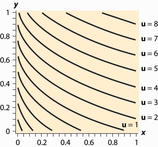
Figure 12.14 Quasilinear isoquants

The procedure for dealing with corners is generally this. First, check concavity of the h function. If h is concave, we have a procedure to solve the problem; when h is not concave, an alternative strategy must be devised. There are known strategies for some cases that are beyond the scope of this text. Given h concave, the next step is to check the endpoints and verify that $h^{\prime }(0)>0$ (for otherwise x = 0 maximizes the consumer’s utility) and $h^{\prime }\left(\raisebox{1ex}{$M$}\!\left/ \!\raisebox{-1ex}{$p_X$}\right.\right)<0$ (for otherwise y = 0 maximizes the consumer’s utility). Finally, at this point we seek the interior solution $h^{\prime }(x)=0\text{.}$ With this procedure, we can ensure that we find the actual maximum for the consumer rather than a solution to the first-order conditions that don’t maximize the consumer’s utility.