This is “Producer Theory: Dynamics”, chapter 10 from the book Beginning Economic Analysis (v. 1.0). For details on it (including licensing), click here.
For more information on the source of this book, or why it is available for free, please see the project's home page. You can browse or download additional books there. To download a .zip file containing this book to use offline, simply click here.


Chapter 10 Producer Theory: Dynamics
How do shocks affect competitive markets?
10.1 Reactions of Competitive Firms
Learning Objective
- How does a competitive firm respond to price changes?
In this section, we consider a competitive firm (or entrepreneur) that can’t affect the price of output or the prices of inputs. How does such a competitive firm respond to price changes? When the price of the output is p, the firm earns profits where c(q|K) is the total cost of producing, given that the firm currently has capital K. Assuming that the firm produces at all, it maximizes profits by choosing the quantity qs satisfying which is the quantity where price equals marginal cost. However, this is a good strategy only if producing a positive quantity is desirable, so that which maybe rewritten as The right-hand side of this inequality is the average variable cost of production, and thus the inequality implies that a firm will produce, provided price exceeds the average variable cost. Thus, the profit-maximizing firm produces the quantity qs, where price equals marginal cost, provided price is as large as minimum average variable cost. If price falls below minimum average variable cost, the firm shuts down.
The behavior of the competitive firm is illustrated in Figure 10.1 "Short-run supply". The thick line represents the choice of the firm as a function of the price, which is on the vertical axis. Thus, if the price is below the minimum average variable cost (AVC), the firm shuts down. When price is above the minimum average variable cost, the marginal cost gives the quantity supplied by the firm. Thus, the choice of the firm is composed of two distinct segments: the marginal cost, where the firm produces the output such that price equals marginal cost; and shutdown, where the firm makes a higher profit, or loses less money, by producing zero.
Figure 10.1 "Short-run supply" also illustrates the average total cost, which doesn’t affect the short-term behavior of the firm but does affect the long-term behavior because, when price is below average total cost, the firm is not making a profit. Instead, it would prefer to exit over the long term. That is, when the price is between the minimum average variable cost and the minimum average total cost, it is better to produce than to shut down; but the return on capital was below the cost of capital. With a price in this intermediate area, a firm would produce but would not replace the capital, and thus would shut down in the long term if the price were expected to persist. As a consequence, minimum average total cost is the long-run “shutdown” point for the competitive firm. (Shutdown may refer to reducing capital rather than literally setting capital to zero.) Similarly, in the long term, the firm produces the quantity where the price equals the long-run marginal cost.
Figure 10.1 Short-run supply
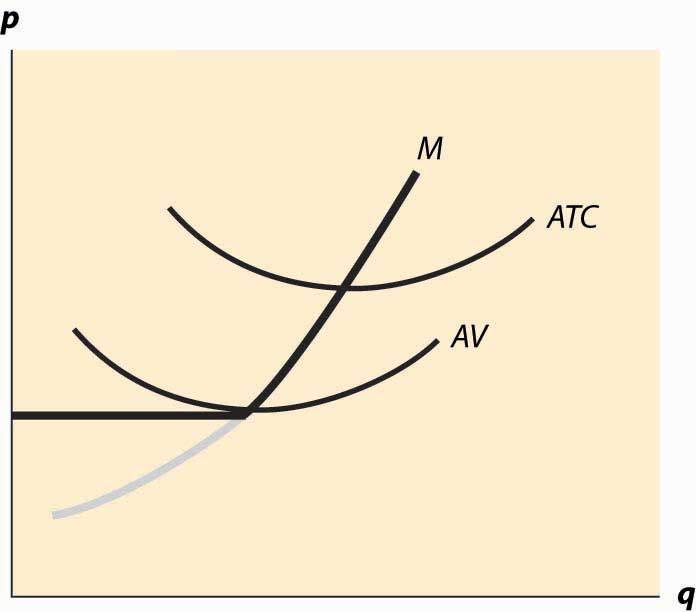
Figure 10.1 "Short-run supply" illustrates one other fact: The minimum of average cost occurs at the point where marginal cost equals average cost. To see this, let C(q) be total cost, so that average cost is C(q)/q. Then the minimum of average cost occurs at the point satisfying
But this can be rearranged to imply , where marginal cost equals average cost at the minimum of average cost.
The long-run marginal cost has a complicated relationship to short-run marginal cost. The problem in characterizing the relationship between long-run and short-run marginal costs is that some costs are marginal in the long run that are fixed in the short run, tending to make long-run marginal costs larger than short-run marginal costs. However, in the long run, the assets can be configured optimally, While some assets are fixed in the short run, and this optimal configuration tends to make long-run costs lower.
Instead, it is more useful to compare the long-run average total costs and short-run average total costs. The advantage is that capital costs are included in short-run average total costs. The result is a picture like Figure 10.2 "Average and marginal costs".
Figure 10.2 Average and marginal costs
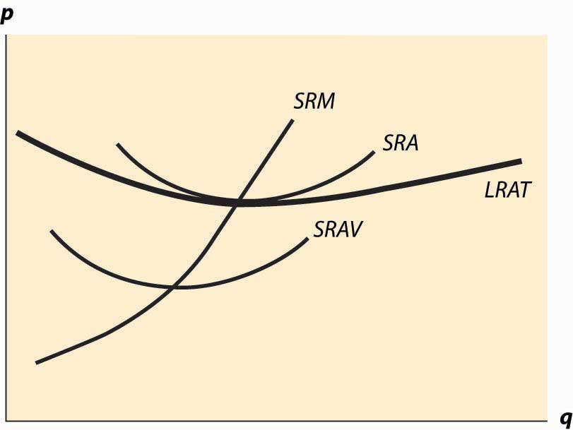
In Figure 10.2 "Average and marginal costs", the short run is unchanged—there is a short-run average cost, short-run average variable cost, and short-run marginal cost. The long-run average total cost has been added, in such a way that the minimum average total cost occurs at the same point as the minimum short-run average cost, which equals the short-run marginal cost. This is the lowest long-run average cost, and has the nice property that long-run average cost equals short-run average total cost equals short-run marginal cost. However, for a different output by the firm, there would necessarily be a different plant size, and the three-way equality is broken. Such a point is illustrated in Figure 10.3 "Increased plant size".
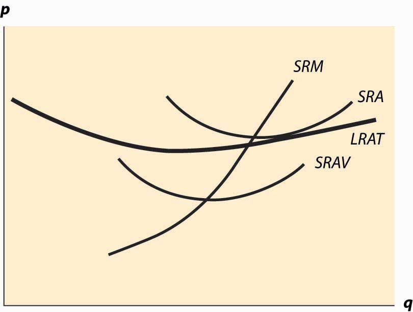
In Figure 10.3 "Increased plant size", the quantity produced is larger than the quantity that minimizes long-run average total cost. Consequently, as is visible in the figure, the quantity where short-run average cost equals long-run average cost does not minimize short-run average cost. What this means is that a factory designed to minimize the cost of producing a particular quantity won’t necessarily minimize short-run average cost. Essentially, because the long-run average total cost is increasing, larger plant sizes are getting increasingly more expensive, and it is cheaper to use a somewhat “too small” plant and more labor than the plant size with the minimum short-run average total cost. However, this situation wouldn’t likely persist indefinitely because, as we shall see, competition tends to force price to the minimum long-run average total cost. At this point, then, we have the three-way equality between long-run average total cost, short-run average total cost, and short-run marginal cost.
Figure 10.3 Increased plant size
Key Takeaways
- The profit-maximizing firm produces the quantity where price equals marginal cost, provided price is as large as minimum average variable cost. If price falls below minimum average variable cost, the firm shuts down.
- When price falls below short-run average cost, the firm loses money. If price is above average variable cost, the firm loses less money than it would by shutting down; once price falls below short-run average variable cost, shutting down entails smaller losses than continuing to operate.
- The minimum of average cost occurs at the point where marginal cost equals average cost.
- If price is below long-run average cost, the firm exits in the long run.
- Every point on long-run average total cost must be equal to a point on some short-run average total cost.
- The quantity where short-run average cost equals long-run average cost need not minimize short-run average cost if long-run average cost isn’t constant.
Exercise
- Suppose a company has total cost given by where capital K is fixed in the short run. What is short-run average total cost and what is marginal cost? Plot these curves. For a given quantity q0, what level of capital minimizes total cost? What is the minimum average total cost of q0?
10.2 Economies of Scale and Scope
Learning Objectives
- When firms get bigger, when do average costs rise or fall?
- How does size relate to profit?
An economy of scaleSituation that exists when larger scale lowers average cost.—that larger scale lowers cost—arises when an increase in output reduces average costs. We met economies of scale and its opposite, diseconomies of scale, in the previous section, with an example where long-run average total cost initially fell and then rose, as quantity was increased.
What makes for an economy of scale? Larger volumes of productions permit the manufacture of more specialized equipment. If I am producing a million identical automotive taillights, I can spend $50,000 on an automated plastic stamping machine and only affect my costs by 5 cents each. In contrast, if I am producing 50,000 units, the stamping machine increases my costs by a dollar each and is much less economical.
Indeed, it is somewhat more of a puzzle to determine what produces a diseconomy of scale. An important source of diseconomies is managerial in nature—organizing a large, complex enterprise is a challenge, and larger organizations tend to devote a larger percentage of their revenues to management of the operation. A bookstore can be run by a couple of individuals who rarely, if ever, engage in management activities, where a giant chain of bookstores needs finance, human resource, risk management, and other “overhead” type expenses just in order to function. Informal operation of small enterprises is replaced by formal procedural rules in large organizations. This idea of managerial diseconomies of scale is reflected in the aphorism “A platypus is a duck designed by a committee.”
In his influential 1975 book The Mythical Man-Month, IBM software manager Fred Books describes a particularly severe diseconomy of scale. Adding software engineers to a project increases the number of conversations necessary between pairs of individuals. If there are n engineers, there are ½n (n – 1) pairs, so that communication costs rise at the square of the project size. This is pithily summarized in Brooks’ Law: “Adding manpower to a late software project makes it later.”
Another related source of diseconomies of scale involves system slack. In essence, it is easier to hide incompetence and laziness in a large organization than in a small one. There are a lot of familiar examples of this insight, starting with the Peter Principle, which states that people rise in organizations to the point of their own incompetence, meaning that eventually people cease to do the jobs that they do well.Laurence Johnston Peter (1919–1990). The notion that slack grows as an organization grows implies a diseconomy of scale.
Generally, for many types of products, economies of scale from production technology tend to reduce average cost, up to a point where the operation becomes difficult to manage. Here the diseconomies tend to prevent the firm from economically getting larger. Under this view, improvements in information technologies over the past 20 years have permitted firms to get larger and larger. While this seems logical, in fact firms aren’t getting that much larger than they used to be; and the share of output produced by the top 1,000 firms has been relatively steady; that is, the growth in the largest firms just mirrors world output growth.
Related to an economy of scale is an economy of scopeSituation that exists when producing more related goods lowers average cost.. An economy of scope is a reduction in cost associated with producing several distinct goods. For example, Boeing, which produces both commercial and military jets, can amortize some of its research and development (R&D) costs over both types of aircraft, thereby reducing the average costs of each. Scope economies work like scale economies, except that they account for advantages of producing multiple products, where scale economies involve an advantage of multiple units of the same product.
Economies of scale can operate at the level of the individual firm but can also operate at an industry level. Suppose there is an economy of scale in the production of an input. For example, there is an economy of scale in the production of disk drives for personal computers. This means that an increase in the production of PCs will tend to lower the price of disk drives, reducing the cost of PCs, which is a scale economy. In this case, it doesn’t matter to the scale economy whether one firm or many firms are responsible for the increased production. This is known as an external economy of scaleAn economy of scale that operates at the industry level, not the individual firm level., or an industry economy of scale, because the scale economy operates at the level of the industry rather than in the individual firm. Thus, the long-run average cost of individual firms may be flat, while the long-run average cost of the industry slopes downward.
Even in the presence of an external economy of scale, there may be diseconomies of scale at the level of the firm. In such a situation, the size of any individual firm is limited by the diseconomy of scale, but nonetheless the average cost of production is decreasing in the total output of the industry, through the entry of additional firms. Generally there is an external diseconomy of scale if a larger industry drives up input prices; for example, increasing land costs. Increasing the production of soybeans significantly requires using land that isn’t so well suited for them, tending to increase the average cost of production. Such a diseconomy is an external diseconomy rather than operating at the individual farmer level. Second, there is an external economy if an increase in output permits the creation of more specialized techniques and a greater effort in R&D is made to lower costs. Thus, if an increase in output increases the development of specialized machine tools and other production inputs, an external economy will be present.
An economy of scale arises when total average cost falls as the number of units produced rises. How does this relate to production functions? We let y = f(x1, x2, … , xn) be the output when the n inputs x1, x2, … ,xn are used. A rescaling of the inputs involves increasing the inputs by a fixed percentage; e.g., multiplying all of them by the constant λ (the Greek letter “lambda”), where λ > 1. What does this do to output? If output goes up by more than λ, we have an economy of scale (also known as increasing returns to scaleSituation that exists when increasing all inputs by the same scalar factor increases output by more than the scalar factor.): Scaling up production increases output proportionately more. If output goes up by less than λ, we have a diseconomy of scale, or decreasing returns to scaleSituation that exists when increasing all inputs by the same scalar factor increases output by less than the scalar factor.. And finally, if output rises by exactly λ, we have constant returns to scaleSituation that exists when increasing all inputs by the same scalar factor increases output by that scalar factor.. How does this relate to average cost? Formally, we have an economy of scale if if λ > 1.
This corresponds to decreasing average cost. Let w1 be the price of input one, w2 the price of input two, and so on. Then the average cost of producing y = f(x1, x2, … , xn) is AVC =
What happens to average cost as we scale up production by λ > 1? Call this AVC(λ).
Thus, average cost falls if there is an economy of scale and rises if there is a diseconomy of scale.
Another insight about the returns to scale concerns the value of the marginal product of inputs. Note that if there are constant returns to scale, then
The value is the marginal product of input x1, and similarly is the marginal product of the second input, and so on. Consequently, if the production function exhibits constant returns to scale, it is possible to divide up output in such a way that each input receives the value of the marginal product. That is, we can give to the suppliers of input one, to the suppliers of input two, and so on; and this exactly uses up all of the output. This is known as “paying the marginal product,” because each supplier is paid the marginal product associated with the input.
If there is a diseconomy of scale, then paying the marginal product is feasible; but there is generally something left over, too. If there are increasing returns to scale (an economy of scale), then it is not possible to pay all the inputs their marginal product; that is,
Key Takeaways
- An economy of scale arises when an increase in output reduces average costs.
- Specialization may produce economies of scale.
- An important source of diseconomies is managerial in nature—organizing a large, complex enterprise is a challenge, and larger organizations tend to devote a larger percentage of their revenues to management of the operation.
- An economy of scope is a reduction in cost associated with producing several related goods.
- Economies of scale can operate at the level of the individual firm but can also operate at an industry level. At the industry level, scale economies are known as an external economies of scale or an industry economies of scale.
- The long-run average cost of individual firms may be flat, while the long-run average cost of the industry slopes downward.
- Generally there is an external diseconomy of scale if a larger industry drives up input prices. There is an external economy if an increase in output permits the creation of more specialized techniques and a greater effort in R&D is made to lower costs.
- A production function has increasing returns to scale if an increase in all inputs by a constant factor λ increases output by more than λ.
- A production function has decreasing returns to scale if an increase in all inputs by a constant factor λ increases output by less than λ.
- The production function exhibits increasing returns to scale if and only if the cost function has an economy of scale.
- When there is an economy of scale, the sum of the values of the marginal product exceeds the total output. Consequently, it is not possible to pay all inputs their marginal product.
- When there is a diseconomy of scale, the sum of the values of the marginal product is less than the total output. Consequently, it is possible to pay all inputs their marginal product and have something left over for the entrepreneur.
Exercises
- Given the Cobb-Douglas production function show that there is constant returns to scale if increasing returns to scale if , and decreasing returns to scale if
- Suppose a company has total cost given by where capital K can be adjusted in the long run. Does this company have an economy of scale, diseconomy of scale, or constant returns to scale in the long run?
- A production function f is homogeneous of degree r if Consider a firm with a production function that is homogeneous of degree r. Suppose further that the firm pays the value of marginal product for all of its inputs. Show that the portion of revenue left over is 1 – r.
10.3 Dynamics With Constant Costs
Learning Objective
- How do changes in demand or cost affect the short- and long-run prices and quantities traded?
Having understood how a competitive firm responds to price and input cost changes, we consider how a competitive market responds to demand or cost changes.
Figure 10.4 Long-run equilibrium
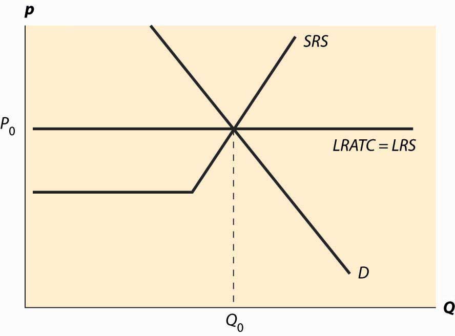
The basic picture of a long-run equilibrium is presented in Figure 10.4 "Long-run equilibrium". There are three curves, all of which are already familiar. First, there is demand, considered in the first chapter. Here, demand is taken to be the “per-period” demand. Second, there is the short-run supply, which reflects two components—a shutdown point at minimum average variable cost, and quantity such that price equals short-run marginal cost above that level. The short-run supply, however, is the market supply level, which means that it sums up the individual firm effects. Finally, there is the long-run average total cost at the industry level, thus reflecting any external diseconomy or economy of scale. As drawn in Figure 10.4 "Long-run equilibrium", there is no long-run scale effect. The long-run average total cost is also the long-run industry supply.This may seem confusing, because supply is generally the marginal cost, not the average cost. However, because a firm will quit producing in the long-term if price falls below its minimum average cost, the long-term supply is just the minimum average cost of the individual firms because this is the marginal cost of the industry.
As drawn, the industry is in equilibrium, with price equal to P0, which is the long-run average total cost, and also equates short-run supply and demand. That is, at the price of P0, and industry output of Q0, no firm wishes to shut down, no firm can make positive profits from entering, there is no excess output, and no consumer is rationed. Thus, no market participant has an incentive to change his or her behavior, so the market is in both long-run and short-run equilibrium. In long-run equilibriumThe point where both long-run demand equals long-run supply and short-run demand equals short-run supply., long-run demand equals long-run supply, and short-run demand equals short-run supply, so the market is also in short-run equilibriumThe point where short-run demand equals short-run supply., where short-run demand equals short-run supply.
Now consider an increase in demand. Demand might increase because of population growth, or because a new use for an existing product is developed, or because of income growth, or because the product becomes more useful. For example, the widespread adoption of the Atkins diet increased demand for high-protein products like beef jerky and eggs. Suppose that the change is expected to be permanent. This is important because the decision of a firm to enter is based more on expectations of future demand than on present demand.
Figure 10.5 "A shift in demand" reproduces the equilibrium figure, but with the curves “grayed out” to indicate a starting position and a darker, new demand curve, labeled D1.
Figure 10.5 A shift in demand
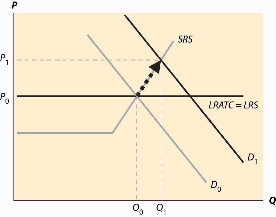
The initial effect of the increased demand is that the price is bid up, because there is excess demand at the old price, P0. This is reflected by a change in both price and quantity to P1 and Q1, to the intersection of the short-run supply (SRS) and the new demand curve. This is a short-run equilibrium, and persists temporarily because, in the short run, the cost of additional supply is higher.
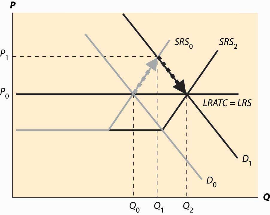
At the new, short-run equilibrium, price exceeds the long-run supply (LRS) cost. This higher price attracts new investment in the industry. It takes some time for this new investment to increase the quantity supplied, but over time the new investment leads to increased output, and a fall in the price, as illustrated in Figure 10.6 "Return to long-run equilibrium".
As new investment is attracted into the industry, the short-run supply shifts to the right because, with the new investment, more is produced at any given price level. This is illustrated with the darker short-run supply, SRS2. The increase in price causes the price to fall back to its initial level and the quantity to increase still further to Q2.
Figure 10.6 Return to long-run equilibrium
It is tempting to think that the effect of a decrease in demand just retraces the steps of an increase in demand, but that isn’t correct. In both cases, the first effect is the intersection of the new demand with the old short-run supply. Only then does the short-run supply adjust to equilibrate the demand with the long-run supply; that is, the initial effect is a short-run equilibrium, followed by adjustment of the short-run supply to bring the system into long-run equilibrium. Moreover, a small decrease in demand can have a qualitatively different effect in the short run than a large decrease in demand, depending on whether the decrease is large enough to induce immediate exit of firms. This is illustrated in Figure 10.7 "A decrease in demand".
In Figure 10.7 "A decrease in demand", we start at the long-run equilibrium where LRS and D0 and SRS0 all intersect. If demand falls to D1, the price falls to the intersection of the new demand and the old short-run supply, along SRS0. At that point, exit of firms reduces the short-run supply and the price rises, following along the new demand D1.
Figure 10.7 A decrease in demand
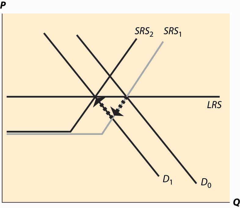
If, however, the decrease in demand is large enough to push the industry to minimum average variable cost, there is immediate exit. In Figure 10.8 "A big decrease in demand", the fall in demand from D0 to D1 is sufficient to push the price to minimum average variable cost, which is the shutdown point of suppliers. Enough suppliers have to shut down to keep the price at this level, which induces a shift of the short-run supply, to SRS1. Then there is additional shutdown, shifting in the short-run supply still further, but driving up the price (along the demand curve) until the long-term equilibrium is reached.
Figure 10.8 A big decrease in demand
Consider an increase in the price of an input into production. For example, an increase in the price of crude oil increases the cost of manufacturing gasoline. This tends to decrease (shift up) both the long-run supply and the short-run supply by the amount of the cost increase. The effect is illustrated in Figure 10.9 "A decrease in supply". The increased costs reduce both the short-run supply (prices have to be higher in order to produce the same quantity) and the long-run supply. The short-run supply shifts upward to SRS1 and the long-run supply to LRS2. The short-run effect is to move to the intersection of the short-run supply and demand, which is at the price P1 and the quantity Q1. This price is below the long-run average cost, which is the long-run supply, so over time some firms don’t replace their capital and there is disinvestment in the industry. This disinvestment causes the short-run supply to be reduced (move left) to SRS2.
Figure 10.9 A decrease in supply
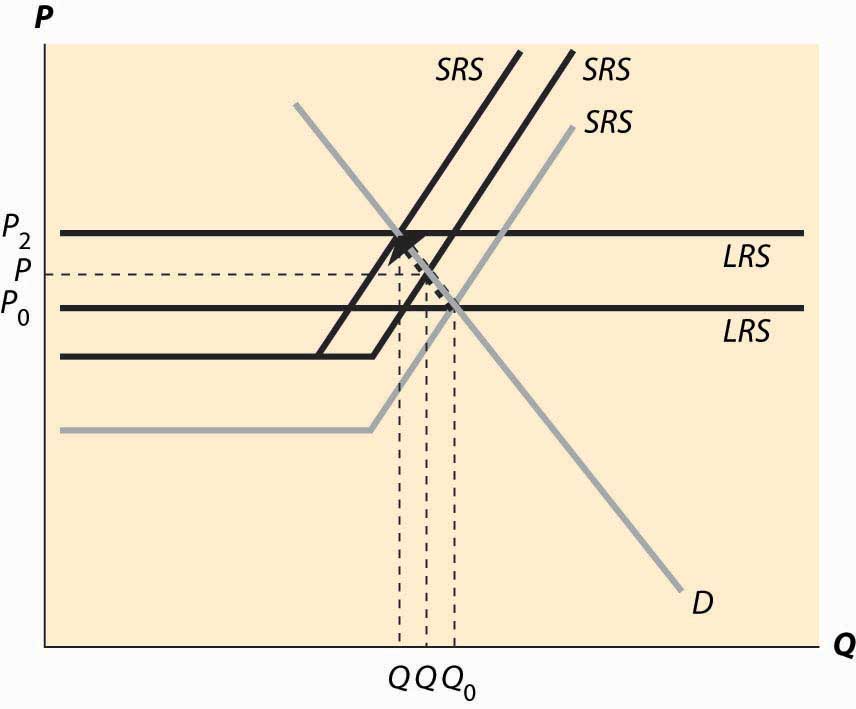
The case of a change in supply is more challenging because both the long-run supply and the short-run supply are shifted. But the logic—start at a long-run equilibrium, then look for the intersection of current demand and short-run supply, then look for the intersection of current demand and long-run supply—is the same whether demand or supply have shifted.
Key Takeaways
- A long-run equilibrium occurs at a price and quantity when the demand equals the long-run supply, and the number of firms is such that the short-run supply equals the demand.
- At long-run equilibrium prices, no firm wishes to shut down, no firm can make positive profits from entering, there is no excess output, and no consumer is rationed.
- An increase in demand to a system in long-run equilibrium first causes a short-run increase in output and a price increase. Then, because entry is profitable, firms enter. Entry shifts out short-run supply until the system achieves long-run equilibrium, decreasing prices back to their original level and increasing output.
- A decrease in demand creates a short-run equilibrium where existing short-run supply equals demand, with a fall in price and output. If the price fall is large enough (to average variable cost), some firms shut down. Then as firms exit, supply contracts, prices rise, and quantity contracts further.
- The case of a change in supply is more challenging because both the long-run supply and the short-run supply are shifted.
10.4 General Long-run Dynamics
Learning Objective
- If long-run costs aren’t constant, how do changes in demand or costs affect short- and long-run prices and quantities traded?
The previous section made two simplifying assumptions that won’t hold in all applications of the theory. First, it assumed constant returns to scale, so that long-run supply is horizontal. A perfectly elastic long-run supply means that price always eventually returns to the same point. Second, the theory didn’t distinguish long-run from short-run demand. But with many products, consumers will adjust more over the long-term than immediately. As energy prices rise, consumers buy more energy-efficient cars and appliances, reducing demand. But this effect takes time to be seen, as we don’t immediately scrap our cars in response to a change in the price of gasoline. The short-run effect is to drive less in response to an increase in the price, while the long-run effect is to choose the appropriate car for the price of gasoline.
To illustrate the general analysis, we start with a long-run equilibrium. Figure 10.10 "Equilibrium with external scale economy" reflects a long-run economy of scale, because the long-run supply slopes downward, so that larger volumes imply lower cost. The system is in long-run equilibrium because the short-run supply and demand intersection occurs at the same price and quantity as the long-run supply and demand intersection. Both short-run supply and short-run demand are less elastic than their long-run counterparts, reflecting greater substitution possibilities in the long run.
Figure 10.10 Equilibrium with external scale economy
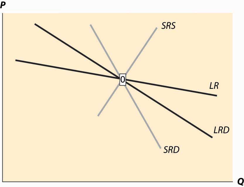
Figure 10.11 Decrease in demand
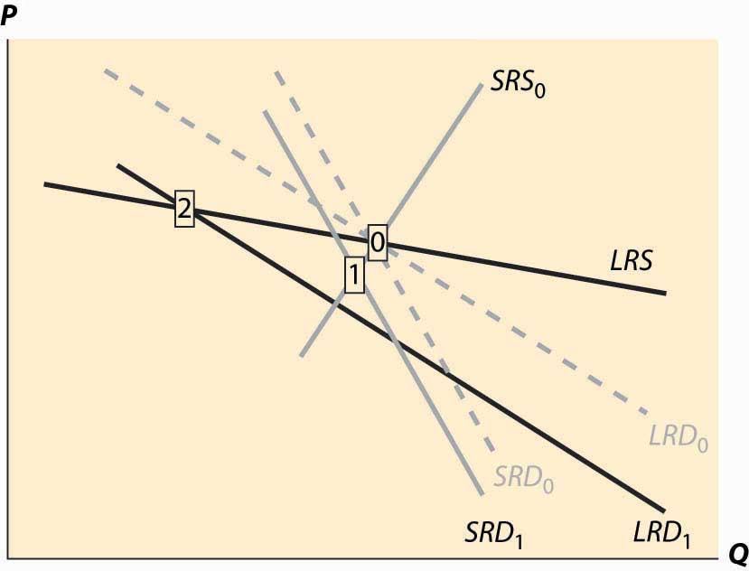
Now consider a decrease in demand, decreasing both short-run and long-run demand. This is illustrated in Figure 10.11 "Decrease in demand". To reduce the proliferation of curves, we colored the old demand curves very faintly and marked the initial long-run equilibrium with a zero inside a small rectangle.The short-run demand and long-run demand have been shifted down by the same amount; that is, both reflect an equal reduction in value. This kind of shift might arise if, for instance, a substitute had become cheaper; but the equal reduction is not essential to the theory. In addition, the fact of equal reductions often isn’t apparent from the diagram, because of the different slopes—to most observers, it appears that short-run demand fell less than long-run demand. This isn’t correct, however, and one can see this because the intersection of the new short-run demand and long-run demand occurs directly below the intersection of the old curves, implying both fell by equal amounts. The intersection of short-run supply and short-run demand is marked with the number 1. Both long-run supply and long-run demand are more elastic than their short-run counterparts, which has an interesting effect. The short-run demand tends to shift down over time, because the price associated with the short-run equilibrium is above the long-run demand price for the short-run equilibrium quantity. However, the price associated with the short-run equilibrium is below the long-run supply price at that quantity. The effect is that buyers see the price as too high, and are reducing their demand, while sellers see the price as too low, and so are reducing their supply. Both short-run supply and short-run demand fall, until a long-run equilibrium is achieved.
Figure 10.12 Long-run after a decrease in demand
In this case, the long-run equilibrium involves higher prices, at the point labeled 2, because of the economy of scale in supply. This economy of scale means that the reduction in demand causes prices to rise over the long run. The short-run supply and demand eventually adjust to bring the system into long-run equilibrium, as Figure 10.12 "Long-run after a decrease in demand" illustrates. The new long-run equilibrium has short-run demand and supply curves associated with it, and the system is in long-run equilibrium because the short-run demand and supply, which determine the current state of the system, intersect at the same point as the long-run demand and supply, which determine where the system is heading.
There are four basic permutations of the dynamic analysis—demand increase or decrease and a supply increase or decrease. Generally, it is possible for long-run supply to slope down—this is the case of an economy of scale—and for long-run demand to slope up.The demand situation analogous to an economy of scale in supply is a network externality, in which the addition of more users of a product increases the value of the product. Telephones are a clear example—suppose you were the only person with a phone—but other products like computer operating systems and almost anything involving adoption of a standard represent examples of network externalities. When the slope of long-run demand is greater than the slope of long-run supply, the system will tend to be inefficient, because an increase in production produces higher average value and lower average cost. This usually means that there is another equilibrium at a greater level of production. This gives 16 variations of the basic analysis. In all 16 cases, the procedure is the same. Start with a long-run equilibrium and shift both the short-run and long-run levels of either demand or supply. The first stage is the intersection of the short-run curves. The system will then go to the intersection of the long-run curves.
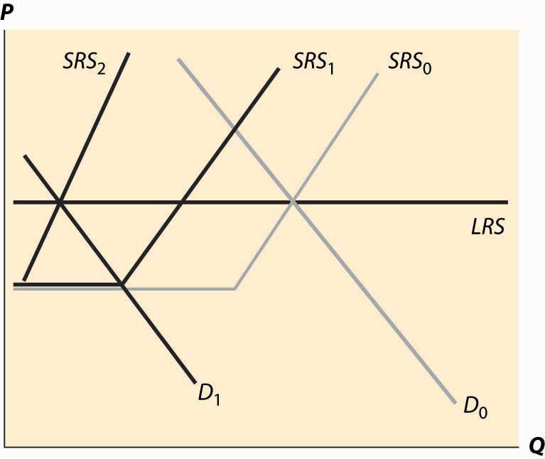
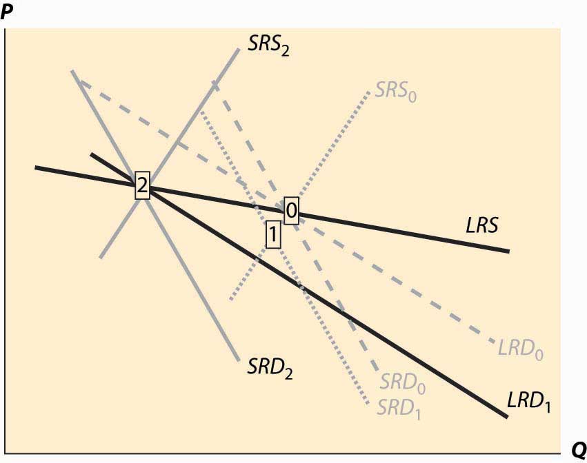
An interesting example of competitive dynamics’ concepts is the computer memory market, which was discussed previously. Most of the costs of manufacturing computer memory are fixed costs. The modern DRAM plant costs several billion dollars; the cost of other inputs—chemicals, energy, labor, silicon wafers—are modest in comparison. Consequently, the short-run supply is vertical until prices are very, very low; at any realistic price, it is optimal to run these plants 100% of the time.The plants are expensive, in part, because they are so clean—a single speck of dust falling on a chip ruins the chip. The Infineon DRAM plant in Virginia stopped operations only when a snowstorm prevented workers and materials from reaching the plant. The nature of the technology has allowed manufacturers to cut the costs of memory by about 30% per year over the past 40 years, demonstrating that there is a strong economy of scale in production. These two features—vertical short-run supply and strong economies of scale—are illustrated in Figure 10.13 "DRAM market". The system is started at the point labeled with the number 0, with a relatively high price, and technology that has made costs lower than this price. Responding to the profitability of DRAM, short-run supply shifts out (new plants are built and die-shrinks permit increasing output from existing plants). The increased output causes prices to fall relatively dramatically because short-run demand is inelastic, and the system moves to the point labeled 1. The fall in profitability causes DRAM investment to slow, which allows demand to catch up, boosting prices to the point labeled 2. (One should probably think of Figure 10.13 "DRAM market" as being in a logarithmic scale.)
Figure 10.13 DRAM market
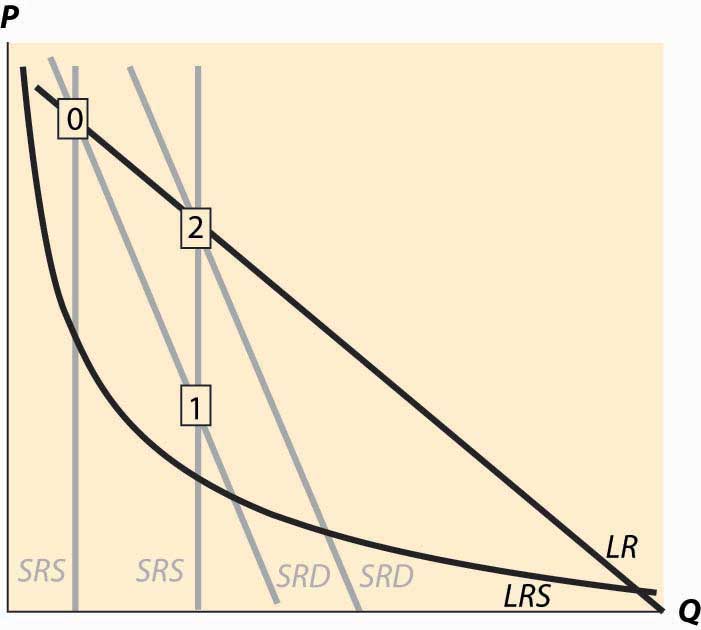
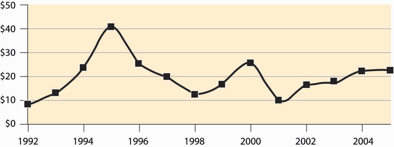
The point labeled with the number 2 looks qualitatively similar to the point labeled with the number 1. The prices have followed a “sawtooth” pattern, and the reason is due to the relatively slow adjustment of demand compared to supply, as well as the inelasticity of short-run demand, which creates great price swings as short-run supply shifts out. Supply can be increased quickly and is increased “in lumps” because a die-shrink (making the chips smaller so that more fit on a given silicon wafer) tends to increase industry production by a large factor. This process can be repeated starting at the point labeled 2. The system is marching inexorably toward a long-run equilibrium in which electronic memory is very, very cheap even by current standards and is used in applications that haven’t yet been considered; but the process of getting there is a wild ride, indeed. The sawtooth pattern is illustrated in Figure 10.14 "DRAM revenue cycle", which shows DRAM industry revenues in billions of dollars from 1992 to 2003, and projections of 2004 and 2005.Two distinct data sources were used, which is why there are two entries for each of 1998 and 1999.
Figure 10.14 DRAM revenue cycle
Key Takeaway
- In general, both demand and supply may have long-run and short-run curves. In this case, when something changes, initially the system moves to the intersections of the current short-run supply and demand for a short-run equilibrium, then to the intersection of the long-run supply and demand. The second change involves shifting short-run supply and demand curves.
Exercises
- Land close to the center of a city is in fixed supply, but it can be used more intensively by using taller buildings. When the population of a city increases, illustrate the long- and short-run effects on the housing markets using a graph.
- Emus can be raised on a wide variety of ranch land, so that there are constant returns to scale in the production of emus in the long run. In the short run, however, the population of emus is limited by the number of breeding pairs of emus, and the supply is essentially vertical. Illustrate the long- and short-run effects of an increase in demand for emus. (In the late 1980s, there was a speculative bubble in emus, with prices reaching $80,000 per breeding pair, in contrast to $2,000 or so today.)
- There are long-run economies of scale in the manufacture of computers and their components. There was a shift in demand away from desktop computers and toward notebook computers around the year 2001. What are the short- and long-run effects? Illustrate your answer with two diagrams, one for the notebook market and one for the desktop market. Account for the fact that the two products are substitutes, so that if the price of notebook computers rises, some consumers shift to desktops. (To answer this question, start with a time 0 and a market in long-run equilibrium. Shift demand for notebooks out and demand for desktops in.) What happens in the short run? What happens in the long run to the prices of each? What does that price effect do to demand?